NatureScot Research Report 1356 - Application of surface motion remote sensing to quantify the condition and trajectory of change of c.680,000 ha of peatland
Published: 2025
Authors: David J Large (1), Andrew V Bradley (2), Emily Mitchell (3), Chris Fallaize (3), Ian Dryden (3), Roxane Andersen (4) and Chris Marshall (4)
(1) Dept. of Chemical and Environmental Engineering, University of Nottingham, Coates Building, Nottingham, UK, NG7 2RD
(2) Nottingham Geospatial Institute, University of Nottingham, 30 Triumph Road, Lenton, Nottingham, UK, NG7 2TU
(3) School of Mathematical Sciences, University of Nottingham, Nottingham NG7 2RD, UK
(4) Environmental Research Institute, University of the Highlands and Islands, Castle Street, Thurso, UK, KW14 7JD
Cite as: Large, D.J., Bradley, A.V., Mitchell, E., Fallaize, C., Dryden, I., Andersen, R., and Marshall, C. 2025. Application of surface motion remote sensing to quantify the condition and trajectory of change of c.680,000 ha of peatland. NatureScot Research Report 1356.
Keywords
bog breathing; surface motion; InSAR; peatland condition; monitoring; change detection; probability
Background
The purpose of this report is to demonstrate and evaluate the use of peatland surface motion, as measured by interferometric synthetic aperture radar (InSAR) over eight consecutive years, and to quantify and report peatland condition and trajectory of change over large areas.
Peatland surface motion is a sensitive indicator of peatland condition and resilience (Howie and Hebda, 2018; Waddington, 2010; Loisel and Gallego-Sala, 2022). It is a mechanical response to changes in water storage that is determined by a range of peatland properties including elasticity (softness/stiffness), water table depth, plant functional type, land use history and topography. It provides a measure of the ability of a peatland surface to rise and fall with the water table (sometimes called ‘bog breathing’) and hence minimise the risk posed by drought and fire. It also gives an indication of the relative ease with which an area of peat will store water and hence the ease with which it may be restored.
This method provides measures of condition based on ground motion that results from the combined effects of ecology, hydrology and mechanics. This view of condition is a different use of the term ‘condition’ to that provided solely by ecological or hydrological measures. It is a view that provides new information about the behaviour of the peatland that enhances our understanding of peatland function and is complementary to ecological and hydrological measures of condition. Importantly it does not replace detailed assessment of peatland ecology or hydrology condition should specific measures of these parameters be required.
A significant advantage of the InSAR technique is the capability to monitor peatland surfaces irrespective of cloud cover, which can be a severe limitation for optical remote sensing methods in Scotland. This advantage permits frequent monitoring of surface location in order to create a time series of surface movement and offers the potential to monitor peatlands objectively at the national scale and over long time periods.
Previous work both in peer-reviewed publications (Alshammari et al., 2018; Alshammari et al., 2020; Bradley et al., 2022; Islam et al., 2022; Marshall et al., 2022) and NatureScot Research Reports (Bradley et al., 2025.; Large et al., 2025; Marshall et al., 2021), demonstrated that measures of peatland condition can be derived from surface motion over areas of 10s to 100s of km2 at 20 m resolution. The most recent method for achieving this uses satellite radar data processed using an interferometric synthetic aperture radar (InSAR) technique in conjunction with time series analysis and statistical machine learning (Mitchell et al., 2024). These methods were developed over a wide range of peatland conditions and geographic settings by sampling the blanket bogs and lowland raised bogs in the Flow Country, Aberdeenshire, Midland Valley of Scotland, and Dumfries and Galloway.
The technique has also been developed to quantify short- and long-term trajectories of change in peatland condition (Mitchell et al., 2025) that are sensitive to the impact of restoration, infrastructure development and drought.
The methods have been developed via funding from NERC (NE/P014100/1; NE/T010118/1; NE/T006528/1), Leverhulme Research Leadership Award (RL-2019-002), NatureScot Peatland ACTION and Forestry and Land Scotland. Much of this research has been supported by RSPB, Plantlife, as well as individual landowners, Highland Rewilding (Bunloit Estate) and Welbeck Estate.
The methods have now reached a point of maturity where they can be automated for large-area deployment, integrated with other datasets (e.g. high-resolution optical imagery, topography) and subjected to large-scale testing against a broad spectrum of known conditions. However, large-area deployment has its own challenges including maintaining the consistency of classified outputs over large areas involving multiple packages of InSAR data, each with its own frame of reference. There is also the question as to whether the current classification reliably extends beyond the settings currently investigated (e.g. to wetter areas or those with greater topographic relief).
Evaluation of the extent to which this method represents a practical solution to peatland monitoring therefore requires results to be generated over a large area. This report presents and evaluates the results of condition mapping and change detection at a large scale. Interpretation of the results is illustrated using twelve case studies.
Main findings
- The project has successfully delivered a data product that quantifies an important aspect of peatland condition and the trajectory of change in that condition over a large area of Scotland.
- The results are data driven, objective, quantitative and grounded in a robust statistical framework and summaries of condition and change are easily extracted from the data products.
- The outputs are complementary to traditional assessment of peatland condition, and the additional information provided can aid in restoration project design and restoration prioritisation.
- The simple classification system used is in principle easily understood and inter-related but in detail requires the person interpreting the data to incorporate contextual knowledge of land management, ecology, weather patterns and other events (e.g. fire, track construction) to understand the results. Maps generated need to be informed by timelines of intervention. It cannot be assumed that a shift to degrading status is necessarily bad if it is a step preceding recovery, following, for example, restoration action.
- In the case studies, most observations appear to correspond to expected or known changes that have occurred on the sites.
- The results provide insights into the different expectations as to how lowland raised bogs and upland blanket bogs respond to restoration.
- The change detection techniques described are particularly useful in rapidly assessing whether interventions are causing a change in peatland behaviour in timeframes far shorter than those over which peatland ecological conditions are expected to change.
Acknowledgements
In addition to NatureScot Peatland Action funding this work, we would like to acknowledge the NatureScot Peatland ACTION Data and Evidence team for supporting this research. The work builds directly on work funded via the NERC Landscape Decisions Grant NE/T010118/1. UHI acknowledges funding from the Leverhulme Trust (RL-2019-002) that supports Chris Marshall.
Abbreviations
Advanced Pixel System using Intermittent Baseline Subset (APSIS)
Interferometric Synthetic Aperture Radar (InSAR)
Intergovernmental Panel on Climate Change (IPCC)
National Vegetation Classification (NVC)
Natural Environment Research Council (NERC)
Object Oriented Data Analysis (OODA)
Plant functional type (PFT)
The International Union for Conservation of Nature (IUCN)
Introduction
The scale and ambition of the Scottish Government investment in peatland restoration requires efficient and cost-effective methods for large area monitoring and reporting of peatland condition. Monitoring and reporting are required to inform peatland restoration priorities, quantify outcomes, and identify and minimise risks. Monitoring and reporting of peatland condition is also a crucial component of balancing the provision of onshore renewable energy on peatland with peat restoration outlined in the new National Planning Framework 4 (Scottish Government, 2023).
To extend and enhance large-scale monitoring and reporting of peatland condition, the University of Nottingham and the University of the Highlands and Islands with support from NatureScot Peatland ACTION have, since 2017, developed objective, quantitative methods that use satellite measures of peatland surface motion to assess peatland condition. This work contributes to the Peatland ACTION Partnership Monitoring Strategy which has the overall aim of assessing the effectiveness of the Partnership’s work to restore Scotland’s degraded peatlands. The InSAR approach developed here sits within the “Supporting Priority: Develop new tools to improve peatland monitoring”.
Alternative optical remote sensing methods for the analysis of peatland have been developed (Lees et al., 2018) over many years. However, the measures derived from optical imagery, although providing a valuable indicator of ecosystem health, have not proved sufficiently sensitive to spatial and temporal changes in peatland condition. Frequent cloud cover also results in a discontinuous and mosaicked optical record.
Methods using backscattered synthetic aperture radar have also been developed to quantify water table depths (Lees et al., 2021; Toca et al., 2022) but struggle to provide improved sensitivity to peatland condition when compared to optical methods (Räsänen, Tolvanen and Kareksela, 2022). The conclusion of Räsänen, Tolvanen and Kareksela (2022) was based on a rigorous statistical analysis of the ability of C-band SAR backscatter, optical and combined methods to predict water table depth over a range peatland conditions and restoration stages. Räsänen, Tolvanen and Kareksela. (2022) observe that although some methods work very well on some sites no single method is suited to all peatland classes and optical methods generally outperformed SAR backscatter. Little advantage was found in combining methods and a generally poorer performance of all methods was noted on restoration sites. One reason for the variable performance of SAR backscatter is the weaker response with increasing water table depth. However, Räsänen, Tolvanen and Kareksela (2022), note that better performance may be possible using longer wavelength L-band SAR. Unfortunately, commercially available L-band data is more expensive than the freely available C-band data from the European Space Agency.
Surface motion, as measured by interferometric synthetic aperture radar, is sensitive to changes in the ecological and hydrological state of the peat observed on the ground (Alshammari et al, 2020; Bradley et al., 2022; Marshall et al. 2022). The reason for this is that surface motion is a direct and rapid response to changes in water storage and therefore displays a strong response to wetting and drying that precedes changes in plant functional type (Mahdiyasa et al., 2023). For example, following rewetting, swelling of the peat and a reduction in the rate of subsidence will occur before changes in vegetation.
Surface motion measures therefore add a new dimension to the analysis of peat condition by providing measures of the physical behaviour of the peat that are unobtainable by other remote sensing methods. Long-term trends indicate whether peat is subsiding, stable or growing. Seasonal amplitudes indicate the softness, water table depth and hence resilience of the peat. Timing of seasonal peaks indicates the water storage capacity and sites of water accumulation within a landscape.
The use of satellite radar has a distinct advantage over optical satellites because the microwave signal penetrates cloud cover providing repeated regular measures all year round. Data is usually acquired for each area every 6-12 days, with the majority of the data acquired every 6 days.
This report summarises the application of these surface motion methods to an area of 12,800 km2 (Figure 1) containing approximately 680,000 ha of peat. The report provides guidance on the interpretation of the data products and illustrates this via twelve case studies. The GIS spatial data outputs of the work are available for download.
If you do download the data, please ensure you read the instruction note available on the webpage prior to exploring the data.
Methods
The surface motion methods used to measure peat condition are grounded in a particular approach to classification and validation. This approach uses a statistical machine learning model to quantify the relationship between peat condition and surface motion. Validation of these models is based on defining the surface motion behaviour of well understood endmember peatland conditions. In the sections that follow, we first define the elements of the approach and then summarise the technical aspects of the methods.
Approach
Underlying processes
Movement of the peatland surface occurs in response to change in the amount of water stored in the peat. Other factors can also cause surface motion, for example emission of large volumes of trapped gas or decay of organic matter. However, in temperate peatland change in water storage is the overwhelming cause. The volume of water stored is the difference between the input and output of water in a hydrological budget. Changes in water storage therefore reflect seasonal, temporal, and spatial variations in this balance. An example of this are seasonal patterns of evapotranspiration which in the UK result in water losses during the summer and gains during the winter causing peat to swell in the winter and subside in the summer.
A change in the quantity of water stored in the peat is reflected in the absolute height of the water table. Please note that as the surface can move this is not the same as water table depth. As the height of the water table increases, water storage increases, pore pressure increases and the peat swells. This response is characteristic of a poroelastic material, and a full technical explanation can be found accompanying the most recent generation of fully coupled ecohydrological-mechanical peatland models (Mahdiyasa et al., 2022, 2023).
The amount of surface motion observed is determined by the change in the height of the water table and the poroelastic properties of the peat which in turn depend on the ecohydrology. The coupling of these properties makes peat resilient in the face of varying weather. For example, the surface of a spongy, elastic peatland will fall synchronously with the water table, peat wetness and associated ecology will be maintained, and oxidation of the peat minimised. It is this coupling of the ecohydrological and mechanical processes that make surface motion a powerful indicator of peatland condition.
Condition and change detection
To account for the effect of variable weather and hence variable hydrology, peat condition is best determined by the behaviour of the peat over multiple years. For example, direct field measurements from 2017 to 2019 illustrated that areas of peat in good condition over the Flow Country collapsed during the 2018 European-wide drought (Marshall et al., 2022). This collapse caused irreversible compaction of the peat, flattening the surface topography, and creating a wetter peatland surface during the winter of 2018/19, which only properly re-established typical surface motion in the winter of 2019/2020. Had measurements only been captured over one year, a full understanding of peat condition would not have been acquired. However, measured over a period of three years or more, the condition was clearly good, and the collapse of the surface was recognised as evidence of peatland resilience rather than evidence of degradation.
As it can take many years for peat condition to change following intervention, there is also value in measuring the trajectory or direction of change in that condition (e.g. a positive change towards better condition or a negative change towards a poorer condition) in response to annual and longer-term events. For example, peat may initially swell following rewetting, indicating that the rewetting has caused a positive change towards a better condition irrespective of whether the ecological condition has shifted markedly or not. Similarly, areas of peat in good ecological condition could be undergoing long-term negative change towards a poorer condition on account of nearby drainage or climate change that are masked by the resilient mechanical behaviour of the peatland.
By combining measures of condition and measures of change we can therefore report both the condition of the peat based on long-term behaviours and its trajectory in response to management activities, wildfire, climate extremes, or weather patterns.
Conceptual models and classification
Our classification scheme is based on conceptual models that link surface motion behaviour to observed condition.
In the field, peat condition is determined by a continuum of variable properties on multiple scales like water table depth, plant functional type, land use history, and topography. A good example of this complexity is the variation of microtopography, water table depth and plant functional type observed on near natural peat (e.g. Belyea and Baird, 2006, Andersen et al., 2011). This complexity makes the exact condition hard to define and subjective although there are clear “endmembers”, i.e. well-understood and easily defined conditions at the extremes of the spectrum of possible conditions.
Based on field observations and the desire to keep things simple, we chose to build the classification scheme around three endmember condition classes that are easily inter-related, and mutually exclusive. Other condition classes can be defined, but with a loss of simplicity. To classify intermediate peatland condition, we use a statistical machine learning method to determine the probability that a measured surface motion signal belongs to a particular endmember class.
The following three endmember classes were chosen:
- Degrading. Peat in an actively degrading condition will subside in response to the removal of water via drains or macropores and associated oxidation of the peat. It may have a variable capacity to store water depending on the extent to which degradation has proceeded. Plant functional types will change as water table depths deepen, with shrub (e.g. Calluna vulgaris) or scrub (e.g. Betula spp., Pinus contorta, Picea sitchensis) becoming increasingly dominant. The characteristic surface motion signals are based on those that correspond to areas of actively draining, clear-felled, and eroding sites.
- Good. Peat in good condition will be wet and resilient. A shallow water table will reduce near surface rates of decay and maintain a typical peatland vegetation cover that is rich in Sphagnum mosses and/or sedges; this vegetation cover also contributes to the elasticity of the peatland. The system will readily store water, and this will be reflected in the high amplitude movement of the surface in response to seasonal variations in water storage caused by evapotranspiration. Over multiple years, the peat surface should appear stable or display evidence of slow growth in line with the slow accumulation of peat. In this context it is worth noting that the linear, “conveyor belt” view of a little bit of peat accumulating each year is unproven and a non-linear accumulation process in which peat goes through periods of accumulation and compaction and decay may be equally likely (Mahdiyasa et al., 2023). The signal associated with this condition is defined based on the range of surface motion signals observed over wet near-natural and long-term restoration areas. These areas sometimes contain pool systems, are wet, spongy, potentially rich in Sphagnum spp. and are widely recognised as representing some of the “best” peatland conditions in the UK. They are a typical target condition for many restoration projects. To be clear, the areas subsequently mapped as belonging to this class are not necessarily in the best ecological condition, but their surface motion shares similar characteristics, and this is indicative of the potential to achieve good ecological condition.
- Stiff. Peat in stiff condition is likely to have a vegetation layer dominated by shrub or grasses. Surface oscillations have a low amplitude on account of the stiff consolidated state of the peat, as well as a relatively deep water table and lack of water storage capacity. It will be typical of well drained environments (e.g. steeper slopes and peatland margins), and the later stage of degradation (when peat has consolidated) including areas of upland peat that have experienced long-term erosion, as well as the transition from peat to mineral soil. Long-term rates of subsidence will be low. Characteristic surface motion signals are based on those found on steeper slopes, areas that have experienced long-term erosion, margins and areas of thin peat tending to mineral soil.
These three endmembers can be seen as being linked in a multi-year cycle of degradation and restoration. Starting with a peat in good condition, drainage will shift the peat into a degrading condition, characterised by rapid subsidence. As drainage proceeds the peat will consolidate and stiffen and Sphagnum spp. will be replaced by grass and/or shrub. Rewetting of the stiff peat will cause it to swell and eventually a near surface layer of new peat will establish. Ultimately, given enough time, in the right landscape setting and with the right type of intervention, plant functional types (PFTs) and resilient surface motion can be restored, returning the peat to a good condition. A somewhat similar cycle drives shorter-term resilience in response to drought, linked to physiological differences between PFT: Sphagnum mosses lack active water regulation mechanisms and are more likely to shut down (bleach, collapse), while vascular plants, with roots and stomata can better control water losses and maintain productivity in times of drought (Sterk et al., 2023). Post-drought, the areas that have collapsed the most will be nearer to the water table, supporting higher growth and productivity from Sphagnum. Classification of the endmember and intermediate conditions is based on the characteristics of the InSAR time series. The time series provides a precise but inaccurate measure of surface motion (Marshall et al., 2022). The signal generated by the Advanced Pixel System using Intermittent Baseline Subset (APSIS) InSAR method correctly captures whether the surface is swelling or subsiding and the relative magnitude and timing of surface oscillations, but underestimates the true surface motion (Marshall et al., 2022). This underestimation may be considered a drawback; however, the significant benefit of the method is the valuable near continuous coverage of the peat surface provided by the APSIS technique. The underestimation is also the reason the method is based on the precision of the signal extracted from the InSAR time series. It is this precise ability of the time series to represent the direction and magnitude of surface motion and hence differentiate peat condition that matters most of all.
What is being classified is a signal extracted from an InSAR time series that represents the pattern of motion (trend, amplitude and timing of seasonal oscillations) of the land surface within an area of approximately 20 x 20 m. This area could be relatively flat and homogenous in terms of vegetation cover, or it could be a combination of gully and plateau areas with varying degrees of erosion and vegetation cover; the extracted signal would be an average of the signals collected within that area.
Change detection is based on change in the pattern of motion between chosen periods (e.g. year-to-year) while condition assessment is based on quantification of the entire pattern of motion over several years. Examples of how patterns of motion are related to condition and change classification are:
- A stable trend with a high amplitude winter peak indicates that peat is swelling and storing water in winter and that the soil or substrate is capable of changing volume in response to water storage. This is indicative of peat in good condition.
- A stable trend and low amplitude or no swelling of the peat in winter peak indicates a limited elastic response and/or little water storage capacity. This is indicative of stiff peat.
- A downward trend indicating subsidence is indicative of degrading peat.
- Negative change is associated with increasing rates of subsidence or decreasing rates of swelling.
- Positive change is associated with decreasing rates of subsidence or increasing rates of swelling.
In making these statements we are assuming that the land surface motion is not being actively influenced by civil engineering works, or movement related to mining activities. However, such influences should be borne in mind if appropriate.
Validation
Validation of these methods requires answers to the following questions:
- Does peatland surface motion relate to the condition of the peat?
- Does the surface motion signal precisely represent the true surface motion of the peatland?
- How do the classified characteristics of the peatland surface motion reflect field observations of spatial and temporal changes in peatland condition?
If the answer to questions 1 and 2 is “yes” then the method is undoubtedly capable of providing information on the condition of the peatland. However, only by knowing the answer to question 3 can this be put to effective use.
With respect to question 1, independent published studies have demonstrated that the surface motion characteristics are related to the condition of the peatland as characterised on the ground by methods such as vegetation-based classification, water level monitoring and management history (Price, 2003; Howie and Hebda, 2018; Morton and Heinemeyer, 2019; Evans et al., 2022). If the InSAR measures are therefore accepted as providing a measure of the surface motion, then the InSAR signals must relate to the condition of the peatland. The reason for this relationship is the well-established coupling between the plant ecology, hydrology, and mechanical behaviour of the poroelastic peat (e.g. Ingram, 1983; Almendinger, Almendinger and Glaser, 1986; Mahdiyasa et al., 2023).
With respect to question 2 it has now been shown by multiple and independent surveys (Marshall et al., 2022; Alshammari et al., 2018; Hrysiewiczet al., 2023; Tampuu et al., 2020) that the InSAR time series provides a precise measure of the surface motion, but that it underestimates the magnitude of the motion. It is therefore precise but inaccurate. Observed signals reliably indicate whether an area is subsiding, stable or growing, and the relative magnitudes of this motion. The observations also show whether one area of peat displays a higher or lower seasonal oscillation amplitude than another. The main limit to these measures is the ambiguity threshold, which is exceeded when the movement between pairs of images exceeds a quarter of a wavelength (>1.39 cm for C-band radar ~5.55 cm wavelength). Movement exceeding 1.39 cm in the 6 or 12 days between successive images used to generate the time series is an extraordinarily high rate of subsidence. Beyond this threshold the method cannot resolve the direction of motion. During the drought of 2018, the ambiguity threshold was briefly exceeded across a localised area of peat known to be in extremely good condition in the centre of the Munsary peatlands (Marshall et al., 2022), but this did not compromise the overall condition classification of this area based on multiannual observations (Bradley et al., 2022).
A key challenge in addressing question 3 is matching a continuum in signal behaviour to continuous change in the mechanical, hydrological and ecological properties that interact to determine surface motion. Consequently, this aspect of validation has evolved incrementally over many years and the stages in this evolution are outlined below.
Statistical validation of the relationship between the InSAR signal and surface motion using a range of approaches has been published for the Flow Country and have included extensive ground truthing (Alshammari et al., 2020, Bradley et al., 2022). Validation methods for the Flow Country were developed in two stages, in both instances using a “blind” validation method where ground-based classification was done in situ without prior knowledge of InSAR-derived classification. First a study was completed using only measures of vegetation in 10 x 10 m quadrats centred on 22 random InSAR pixels within the Flow Country (Alshammari et al., 2020). Subsequent measures used land use and land use history, plant functional type, topography, and drainage, with site visits to and data recorded in over 200 discrete landscape “polygons” larger in size (0.3-0.6 km2) (see details in Bradley et al., 2022).
Following these earlier studies, the probability classification method was designed (Mitchell et al., 2024), and initial validation was applied to the sub-site areas analysed in detail in Bradley et al., 2022, where it reliably reproduced classification of areas known to be in good and degraded condition (Mitchell et al., 2024). The conclusion from this work was that the classified InSAR signals reliably identify peat endmembers in good and degrading condition. At this stage, a third class dominated by shrubs and/or areas tending to mineral soil was recognised as representing stiff peat and this was characterised in the work that followed.
A further advancement of the validation method was incorporating a measure of softness, a much more direct link to the poroelastic properties of the peat. This was applied to an area in Dumfries and Galloway that included much of Cairnsmore National Nature Reserve (Bradley et al., 2025). However, application to Cairnsmore, as reported, did not go to plan due to lack of clarity on field definitions (size of area to look at, differences between stiffness categories, mutually exclusive categories). Further, it became apparent that the field measures developed from the Flow Country experience had not been developed to target what turned out to be a narrower range of more degraded and Molinia dominated ecology encountered at Cairnsmore. Consequently, both methods required further refinement. Despite this a statistical separation method (linear discriminant analysis) applied to the small dataset gathered in the field, illustrated that the InSAR conditions (particularly degrading and good conditions) could be reliably separated. Additionally, both the original method (Bradley et al., 2022) and the probability method correctly identified the same degrading areas and areas known to contain stiff peat (Mitchell et al., 2024).
The change detection method was initially validated using a case study of the Camilty forest to bog restoration site in West Lothian. In this case study it correctly identified that the restoration site included twenty of the fifty most changed pixels out of forty thousand pixels within the study area, and that all pixels on the site displayed varying degrees of change following intervention to restore the site. The method was further trialled using a wide range of peatland restoration sites and methods used in the Dalchork Forest and Whitelee Windfarm (Mitchell et al., 2025). In this evaluation, most sites displayed a strong positive response following restoration and different restoration methods were shown to be more drought resilient (i.e. less prone to display a negative response during periods of drought) than others.
In summary,
- Methods reliably separate endmember conditions, as demonstrated by extensive and robust field-based validation.
- Statistical validation has been published in the peer reviewed literature, with reviewers commending the scale of the ground truthing efforts.
- The ability of condition mapping methods to capture intermediate conditions has been thoroughly assessed on a wide range of restoration sites.
What the method does not do and relationship to ecological measures of condition
The method and classification scheme used in this report do not provide a substitute for detailed habitat analysis. Specific condition classes defined using the methods in this report may correspond to more than one ecological state or habitat. For example, within the complex system that defines a blanket peatland, fens and mesotope centres which are both wet, dynamic and resilient may be classified as being in the same condition despite the habitats being quite different. Within blanket peat systems whether fen or otherwise swelling is expected in the winter months with drawdown in spring and summer. As such similar behaviours will be indicative of the response to water storage and hence condition. While fens are hydrologically distinct components of the blanket mire landscape the differences are not sufficient to disrupt the expectation that like the surrounding bog they will swell in the winter and subside in the summer due to variations in evapotranspiration. Substantial deviations from this behaviour would only be expected in fens that are supplied via deep aquifers when a notable offset in the timing of recharge and discharge is possible. In blanket peatland and associated upland slopes lateral flow of water is rapid and shallow so substantial offsets between recharge and discharge are not expected.
In terms of restoration the classifications presented may indicate that a peat is in good condition when the ecology would indicate otherwise. However, it is unlikely a peatland would evolve into a good ecological condition without being classed as being in good condition by the InSAR method. So, whilst the InSAR classification may identify the good class as being present, the area could still be targeted for restoration in order to revegetate any areas of bare peat that may be present; the good classification would increase confidence that the works could recover the area to good ecological condition.
If a detailed ecological analysis is required other methods must be used. The methods presented here are complementary to ecological methods, both providing a different, and important view of peatland function. For example, a peatland may appear be in good ecological condition yet be losing water and subsiding, with the mechanical adjustment of the surface buffering the depth to the water table.
Technical detail of methods
Definition of area of peat
Data is reported for the area defined as containing peat in the Carbon and Peatland 2016 map layer (NatureScot, 2016). Classes 1, 2, 3 and 5 were used as they are identified as containing predominantly peat or peaty soils. It should be noted that Class 5 covers areas identified as peat soil but not containing peatland vegetation, and in many cases may include areas of forestry on peat soil.
InSAR data
InSAR time series of surface motion were purchased from Terra Motion for an area of approximately 12,800 km2, half of which covers the Midland Valley and half the Flow Country and part of the Northern Highlands (Figure 1). The data is for the period 11th May 2015 to 8th January 2023. Terra Motion generate the time series, from Sentinel-1 imagery, using their APSIS InSAR technique, developed from the intermittent small baseline subset technique (Sowter et al., 2013; Sowter et al., 2016, Bradley et al., 2022). This data supplier was chosen as their APSIS method provides near continuous coverage over rural areas.
A total of forty tiles were provided (Figure 1). Tiles for the northern area are labelled N01 to N026, tiles for the southern area S017 to S029 and one separate tile was generated for Islay and is labelled S000.
Within each tile, time series are provided representing the change in surface motion over time within each, approximately, 20 x 20 m pixel. This is a higher resolution than the 90 x 80 m pixel resolution used in previous work with Sentinel-1 data (e.g. Bradley et al., 2022). However, the InSAR processing method used to generate the data is identical. Higher resolution analysis was chosen as this was considered more appropriate relative to the scale of typical restoration projects without being unmanageable from a data handling perspective.
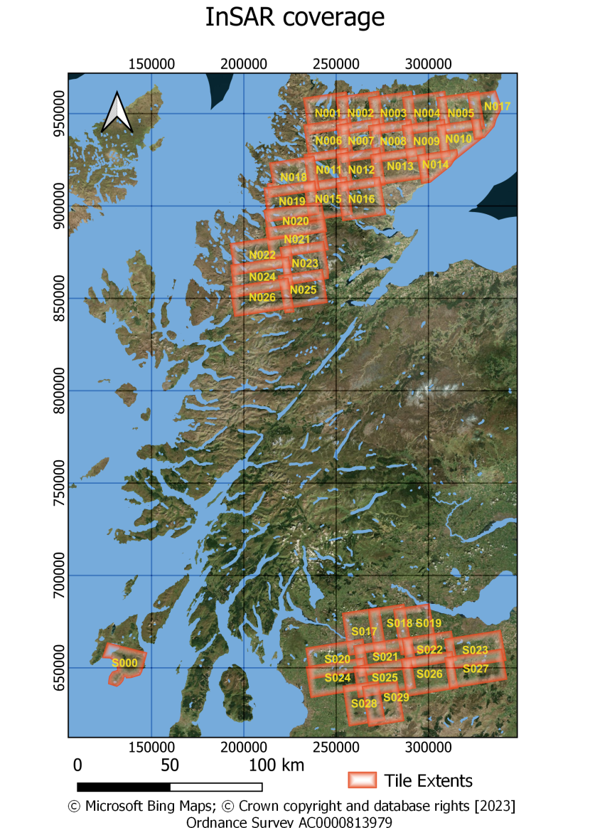
Figure 1: Map showing the distribution of the InSAR data tiles used in this study. Each tile is labelled with the corresponding code provided by the data supplier.
Click for a full description
Overview
Here, we briefly describe the two main stages in the process of going from the raw data (the InSAR time series data at each location/pixel), through to output (condition mapping complete with probabilities, and change detection), to provide context for the more detailed discussion in the following sections.
The first stage is preprocessing of the raw InSAR time series. These time series measure surface motion every 6 or 12 days. Each raw time series is processed (further described below) to extract two measurements – one measuring the behaviour of the overall trend of the series, and one measuring the oscillatory behaviour. These two measures are what we refer to as the “metrics” or “metric data” - it is the data, derived from the raw series, which we then go on to use in the statistical procedures for condition mapping and change detection.
The second stage is to then use statistical models to perform either of the desired tasks (condition mapping/change detection), with the data to be modelled being the metric data extracted from the raw series. These methods are explained in more detail below.
Data pre-processing
For both condition mapping and change detection, time series from Terra Motion are first individually smoothed to capture general behaviour of the series. (The technical name for the type of smoother used is spline interpolation.) There are two main reasons for doing this:
- Although surface motion is recorded every 6 or 12 days, in reality this is a continuum. In theory, the surface motion could be recorded continuously, and we just happen to have measurements at certain time intervals. Mathematically, we think of the surface motion as a function of time – that is, at any point in the time continuum, there is a value of the surface motion series. Smoothing allows us to estimate the surface motion function at any point in time, not just the ones we have observed data for.
- In reality, even at the points in time where we have observed the surface motion, the data are subject to noise. Smoothing allows us to “smooth out” the noise and extract the underlying signal.

Figure 2: A) raw time series. B) the series in A and a highly smoothed curve fitted to it. C) a less-smoothed curve, retaining the seasonal oscillations. D) seasonal oscillations extracted without the trend (the smoothed curve in B minus that of C).
Click for a full description
Examples of the smoothing processes used during data processing. The top left plot shows an example of a raw time series. The top right plot shows this series along with the highly smoothed curve fitted to it. It can be seen that seasonal fluctuations have been smoothed out, leaving a longer-term overall trend. The bottom left plot shows the less-smoothed curve, which retains the seasonal oscillations: this can be thought of as a combination of the longer-term trend plus the oscillations. Finally, to extract the oscillations without the trend, we subtract the overall trend from the “trend + oscillations” curve, the result of which can be seen in the bottom right plot.
In practice, when applying a smoother, the user has a choice of how much smoothing to apply. One can think of the process as a sliding window: the value of the smoothed series at any one point in time will be an average of all the observed data points in a window either side of the time point in question. If this window is wide, data from a relatively long time before and after this point will be averaged out. This is high smoothing, and the effect will be that local fluctuations are smoothed over and the result will be a very smooth, flatter curve. If a narrower window is chosen (less smoothing), only data relatively close (in time) to the point in question is averaged, and the result is a “wigglier” curve. The amount of smoothing is controlled by a smoothing parameter, chosen by the user, which quantifies the timescale on which the smoothing is applied (i.e. relating to the width of the sliding window).
We know that the peat surface motion contains signals on (at least) two main scales: longer timescales (overall trend) and shorter timescales (seasonal oscillations). Thus, we applied two separate smoothers to the raw time series, with smoothing parameter values chosen to match these timescales.
Examples of this smoothing process can be seen in Figure 2. The top left plot shows an example of a raw time series. The top right plot shows this series along with the highly smoothed curve fitted to it. It can be seen that seasonal fluctuations have been smoothed out, leaving a longer-term overall trend. The bottom left plot shows the less-smoothed curve, which retains the seasonal oscillations: this can be thought of as a combination of the longer-term trend plus the oscillations. Finally, to extract the oscillations without the trend, we subtract the overall trend from the “trend + oscillations” curve, the result of which can be seen in the bottom right plot.
The following methods use the smoothed functions for the trend and the oscillations separately to address their respective posed problems. Condition mapping methods will require both the trend and oscillation functions since seasonal oscillatory behaviour in addition to long-term degradation have been found to be indicative of peatland condition. For this report, change detection will focus on the change of long-term trend only.
To account for potential movement in the reference point of each InSAR tile the mean time series of all pixels not within areas classed as peat was subtracted from all pixels in areas classed as peat. This approach assumes that the mean gradient of the trend in time series from mineral soils, hard surfaces and areas of more marginal peatland across a whole tile should be zero. If it is not then it represents movement of the InSAR reference point for which a correction should be made. By doing this, excellent agreement was obtained between results in neighbouring tiles.
Condition mapping methods
Condition mapping finds probabilities of peatland condition for each peatland location based on characteristics of the trend and oscillation smoothed functions.
It is essential that the metric based on the trend function can capture whether the average surface motion across the series was declining. This is a key indicator when identifying degrading peatland. We use the average gradient across the period for this metric. The metric based on the oscillation function needs to capture both the scale and the timing of the oscillations; large oscillations with winter peaks have been found to be indicative of soft peatlands and small summer peaks have been found to be indicative of stiff peatlands. To split these peatland conditions, we find how far away each oscillation function is from a regular sine wave which peaks in the winter. Soft peatlands will have a smaller distance from the sine wave compared to stiff peatlands, which would have a much larger distance from the sine wave. Peatlands between these two cases could become either of these cases, usually because of much smaller oscillations due to degradation.

Figure 3: Graph illustrating data processing of an oscillating signal. The black line is the sine template to which other signals are compared and the coloured lines are example signals. Information on the analysis method is in the Long description.
Click for a full description
Examples of the type of oscillation curves observed. The x-axis is time and the y-axis is a dimensionless measure of the relative displacement of the surface. The black line is the sine template. This has regular annual peaks in the winter and troughs in the summer. The oscillation measure is calculated for each observed oscillation curve as follows: for each point in time, measure the vertical difference between the observed curve and the sine template. Then, sum up all of these differences over all time points to get an overall distance between the observed oscillation curve and the template.
The blue curve in the plot is a close match to the sine template. It has regular winter peaks of a relatively high magnitude, and thus the sum of vertical distances between the blue curve and the since template is relatively small. Thus, a small value of our oscillation measure corresponds to behaviour consistent with peat in good condition. The green curve, whilst exhibiting regular oscillations of a relatively high magnitude, is out of phase with the template (the peaks are occurring in the summer). Hence, the sum of vertical differences between the green curve and the template is large. Thus, a larger value of our oscillation measure is indicative of stiffer peat (peaking in the summer). The red curve exhibits an irregular oscillatory pattern, with a mix of small summer peaks or even missing out a peak. Again, this will produce a larger distance from the template.
Figure 3 shows examples of the type of oscillation curves observed. The black line is the sine template. This has regular annual peaks in the winter and troughs in the summer. The oscillation measure is calculated for each observed oscillation curve as follows: for each point in time, measure the vertical difference between the observed curve and the sine template. Then, all these differences are summed over all time points to get an overall distance between the observed oscillation curve and the template. (Technically, we compute the “Euclidean distance” between the template and each observed curve.)
The blue curve in the plot is a close match to the sine template. It has regular winter peaks of a relatively high magnitude, and consequently the sum of vertical distances between the blue curve and the since template is relatively small. Thus, a small value of the oscillation measure corresponds to behaviour consistent with peat in good condition. The green curve, whilst exhibiting regular oscillations of a relatively high magnitude, is out of phase with the template with peaks occurring in the summer. Hence, the sum of vertical differences between the green curve and the template is large. Thus, a larger value of the oscillation measure is indicative of stiffer peat. The red curve exhibits an irregular oscillatory pattern, with a mix of small summer peaks or even missing out a peak. Again, this will produce a larger distance from the template.
Given the two metrics (based on trend and oscillations) found for each peatland location and the assumption of three classes (good, stiff and degrading), we set endmembers to reflect peatland condition. These can be thought of as being the central member of the distribution of these metrics within each class. Degrading peatland has an endmember with a large negative trend metric regardless of the oscillation metric (i.e. distance from the idealised sine wave): good/wet peatland has an endmember with a less negative trend metric with a small oscillation metric (close to the winter peak sine wave) and stiff peatland with a less negative trend metric and large oscillation metric. These endmembers are semi-supervised from the knowledge of peatlands in Dalchork and the Flow Country.
A sample of metrics from the Dalchork region is shown in Figure 4. (Note that the measures have been standardised to have mean zero: thus, large negative oscillation measures correspond to the smallest distances to the sine template, i.e. the “good” peatland.) To find the probabilities based on the endmembers, we assume the distribution of the two metrics within each class follows a gaussian probability distribution in two dimensions (since there are two metrics). We assume the variance (spread) of the distribution of metrics is the same for each class, and the centres of each class reflect the respective locations of each distribution in this two-dimensional space. In other words, the centres represent a “central” pair of metrics for each class, not an extreme endmember. The contours represent “circles of constant probability” for each class in this two-dimensional space, analogous to contours of constant height for ordinary maps. The centre of each distribution contains the most probability mass, and then the concentric circles represent contours of decreasing probability mass as one moves away from the centre.
It is important to note that these distributions represent the spread of the metrics within each class (with the most being in the centre). They do not represent the probability of being in each class for any point in this two-dimensional space. For example, given a point is observed to be in the extreme left of the plot, it is extremely likely that this is from the degraded class – even though this is somewhat in the outer reaches of the distribution of that class, its relative probability compared to the other two is very large (this is an example of conditional probability – even though being over in the outer left of the plot is a rare event, once we have observed it, it is the relative probability of the three classes which matters). Conversely, a point close to the centre of the degraded class could still reasonably be from any three of the classes. The procedure for computing the relative probabilities is further described below.
The centres and variance parameters were calibrated by fitting distributions to observed metric data from the Dalchork and Flow Country regions, where there is known to be an approximately equal mix of peat representing the different classes. The calibration determined parameters which:
- result in the fitted distributions matching the observed data well;
- give sufficient separation between the classes;
- give sufficient spread so that there is overlap between distributions. This in turn will produce smooth transitions in probabilities between the classes where the metrics fall in borderline regions between classes in the two-dimensional metric space.

Figure 4: Graphical representation of the overlapping probability distributions of the three classes. Black circles are a sample of metrics from the Dalchork region. Concentric circles represent contours of constant probability around each class.
Click for a full description
Graphical representation of the overlapping probability distributions of the degrading, wet and stiff classes. A sample of metrics from the Dalchork region. The x-axis is a dimensionless measure of trend with negative values indicating subsidence and positive values growth. The y-axis is a dimensionless oscillation metric. Note that the measures have been standardised to have a mean of zero: thus, large negative oscillation measures correspond to the smallest distances to the sine template, i.e. the good peat. To find the probabilities based on the endmembers, we assume the distribution of the two metrics within each class follows a gaussian probability distribution in two dimensions. We assume the variance (spread) of the distribution of metrics is the same for each class, and the centres of each class reflect the respective locations of each distribution in this two-dimensional space. Thus, the centres represent a “central” pair of metrics for each class, not an extreme endmember. The contours represent “circles of constant probability” for each class in this two-dimensional space, analogous to contours of constant height for ordinary maps. The centre of each distribution contains the most probability mass, and then the concentric circles represent contours of decreasing probability mass as one moves away from the centre.
Given the metric data derived from the time series at any given pixel, it is of course unknown what the class of the site really is. Our task is to classify, along with a measure of uncertainty, the pixel based on these observed metric values alone. The relative likelihood that these metric values would be observed from each of the three classes is computed using the fitted distributions for each class, which in turn can be rescaled to give a probability for each of the classes. Thus, a pair of metrics which lies in a borderline between two or three of the classes will have approximately equal relative likelihood contribution from these classes, and hence there will be significant probability it came from two or more of the classes, thus giving rise to uncertainty as to the true class. Conversely, a pair of metrics which lands firmly within the distribution of just one of the classes will have relative likelihood dominated by this class, and hence a probability of almost 1 of being from that class.
Hence, by assigning a site to the class with the highest probability, the machine learning framework enables the generation of a classification system. Alongside this, it also gives a measure of uncertainty in the classification by providing a probability associated with each of the three classes.
Interpretation of condition maps
Definitions of the three endmember condition classes is provided in Table 1 along with examples of situations that could confound the classification.
Maximum probability and probability maps have been produced for the first four years of data and the last four years. Maximum probability maps provide a clear and simplified overview of condition. The classification scheme for the maximum probability maps indicates which condition is most likely to occur at each site: namely degrading, good or stiff. However, this view comes with a loss of transitional detail which is extremely useful when considering gradational changes on a given site. For sites where conditions are far from any of the three endmember classes, the maximum probability could be as low as 0.34 and this will only be apparent on the probability maps.
Probability maps provide further detail on how likely each class is to occur at the site. The classification scheme for these plots uses probabilities which are equally spaced with 0.2 spacing between 0 and 1 for each class. The probabilities between the three classes will sum to one. Probabilities close to zero indicate the class is not likely to occur at the site. Probabilities close to one indicates the site will almost certainly belong to that class. This enables comparison of condition between these periods of time, giving an insight into change in condition. However it still lacks detail on scale of change.
| Class Descriptor (map colour) | Description of surface motion | Direct interpretation | Typical example | Other situations and interpretations | Potentially confounding situations |
|---|---|---|---|---|---|
| Good (Blue) | High amplitude seasonal oscillations with stable to rising, potentially oscillatory, multiannual trend. | Dynamic surface swelling in winter in response to water storage in soft spongy peat. Indicative of resilient behaviour as the surface can adapt to the position of the water table. If not in ecologically good condition these areas are likely to be more responsive to restoration on account of their natural tendency to hold water. | Near natural or rewetted peatland with a shallow water table and soft to spongy surface, e.g. near natural sphagnum peat. | Any area that is soft and displays winter swelling which may include: - Gullies between peat hags that hold water in winter, are not actively subsiding and potentially display signs of recovery. - Wet peat soils under forestry | Areas where the surface motion is controlled by other process that do not conform to our conceptual models. This may include: - Tilled farmland. - Fens in which the water levels are artificially controlled. - Fens fed by deep groundwater where the timing of discharge is not determined by simultaneous seasonal hydrology. - Areas influenced by tides - Periods of sustained frost resulting in frost heave (swelling) of the surface. This is more likely at higher altitudes subject to prolonged freezing over periods of 1 month or more. |
| Stiff (Green) | Low amplitude oscillations in winter. Stable trend. | Non-dynamic surface indicative of stiff consolidated peat. | Peat on steeper slopes, at margins or on peat hags that have experienced long-term erosion and consolidation. | Any stiff substrate including: - Peat tending to mineral soil - Mineral soil - Rock - Consolidated peat under floating roads - Consolidation by vehicles | - |
| Degrading (Black) | Sustained subsidence in the trend, possibly at variable rates, with or without evidence of seasonal oscillations. | Active subsidence on account of loss of water and/or oxidation of the peat and/or active erosion. | Peat that is actively subsiding on account of drainage and/or erosion. | Any cause of subsidence on peat: - Compaction due to infrastructure e.g. floating roads - Subsidence due to vehicles - Subsidence due to mass movement (the vertical component of creep or landslide) | Subsidence due to processes not acting on or within the peat e.g.: - Mine subsidence - Landfill |
Change detection methods
Change detection identifies whether there is change in the surface motion between two sequential time periods and a measure of the scale of change. To find a measure which captures change, we first take the smoothed trend function again and find the average gradient for each period. Since interest is in capturing change, the change metric is the difference between the two average gradients for the two time periods. This is repeated for all sites. Those sites with a large positive change metric can be said to have large positive change occur between the time periods, such as a positive response to restoration. A large negative change metric can be said to have a large negative change between the time periods, such as response due to drought.
Interpretation of change maps
Change maps indicate the direction or trajectory of change in peat condition between two periods of observation. The change detection measure is split into five classes:
- large negative (below the 10th percentile)
- slight negative (between the 20th and 10th percentiles)
- not significant (between 20th and 80th percentiles)
- slight positive (between the 80th and 90th percentiles)
- large positive (exceeding the 90th percentile).
The percentile ranges chosen may be adjusted by the user to be more or less sensitive to change. However, slight changes in peat occur naturally and regularly so we have purposefully chosen the ranges to highlight more meaningful change as might be expected from management interventions. The sequential change maps display year on year changes in trajectory whereas the map of overall change compares the first and last four years in the total period of observation. Both have their uses, and both are best understood when contextualised by management or meteorological knowledge. For example, sites in good condition should subside during a drought (negative change) and swell during wetter periods (positive change), the net effect being that one balances the other or that positive change is more dominant demonstrating the resilience of the peatland. Positive change should also follow restoration, although the timescales for this may vary, and evidence of this was used to validate the change detection method (Mitchell et al., in 2025). Similarly, negative change should follow installation of drains and is widely observed after fire and the disruptive processes of felling plantations. It is because change happens due to both natural and management interventions that the contextual information is important if observations of change are to be understood.
Finally change, particularly annual change, need not indicate that the condition of the peat has changed sufficiently to merit a change in condition classification. So, for example, initial swelling of the peat following restoration will produce a positive change but does not instantaneously produce a soft resilient, near natural peat in good condition.
The value of the change measure is really in communicating that the trajectory of the peatland has changed following some management intervention in a way that may ultimately lead to a change in condition. So, when a landowner undertakes peatland restoration work, change detection gives an early indication that the process is working, or similarly could be used to demonstrate that land management is having the opposite effect before the condition of the peat is profoundly altered for the worse.
Overlaps and preparation of the final maps
To eliminate possible edge effects that occur close to margins of InSAR data tiles a 1 km margin was removed from each tile after processing by the change detection and probability methods. The exact area used from each tile was then based on distance from the edge of the map with the chosen pixels being those furthest from the edge. This resulted in minimal contrast between adjacent maps, however it should be noted that on account of differences in InSAR reference points and exact conditions of satellite data acquisition some contrast does occur. Contrasts across tile boundaries, where they exist, could have been removed by averaging however this only disguises the join and we feel that in these circumstances it is better to be aware of potential uncertainties.
FAQs
- Are the chosen endmembers sufficiently representative of peat from different areas?
If objectivity is to be maintained, then what matters most is that well recognised endmembers are chosen and not varied on a regional basis. By doing this, classifications can be meaningfully compared. The argument can also be turned around and the question posed as to what characteristics should a peat in good condition have? If these characteristics include, for example, ‘good’ being soft, wet and resilient while ‘degrading’ indicates peat subsidence, then the classification should apply even if the peatland in question is not ecologically identical to those used to define the endmember.
This signal-based based method based on characteristic endmember behaviours is also more objective than trying to define complex intermediate states of peatland condition based on a wide range of variables.
- What is the relationship of the classification to water table depth?
While there is no doubt that a sustained shallow water table is a characteristic of peat in good condition the classification is based on the mechanical behaviour associated with sustained shallow water table depths. An example of a contradiction that can arise is when restoration produces a shallow water table in stiff peat and dynamic surface motion has yet to establish. The question is really whether this peat should be in good condition or not. In our definition the peat would be classed as stiff and only classed as good when resilient mechanical behaviour (i.e. a return of seasonal oscillations) is established.
- Is stiff peat a near natural condition or the result of degradation?
This very much depends on situation within a landscape. In areas that are naturally well drained e.g. steeper slopes and margins, stiff peat is the near natural condition and, in this setting, would be an appropriate target state following restoration. Whereas in flatter central parts of the peatlands that should be poorly drained, stiff peat is indicative of past degradation (e.g. drainage) leading to consolidation.
- Are the endmember classes represented by a single set of values?
No, endmember classes are distributed over a range of values described by probability (Gaussian/normal) distributions for each class. Given a particular set of measures, these distributions can then be used to derive the probability these measures belong to each of the classes. This is elaborated upon in "technical details”.
- What impact does thick vegetation have on the InSAR data?
Terra Motion, providers of the InSAR data, have provided the following information:
“Thick vegetation is a source of diffuse scattering for a C-band radar sensor. Diffuse scattering is, by its nature, random, and so it is expected that thick vegetation will have a very low coherence and therefore be excluded from any InSAR analysis. In reality, any vegetation canopy is complex and may certainly contain large areas of diffuse scattering but there are also areas where the radar signal penetrates, and specular reflection occurs which gives high coherence and is therefore highly suitable for InSAR. These are often areas where the radar signal finds a gap in the canopy and bounces from ground to trunk, giving a strong corner-reflector-like response. These high-quality areas are the focus of the APSIS method, and the reason APSIS can give reliable results in vegetated areas where other InSAR methods fail. For example, in an analysis of a mixed forest/agricultural area in the UK, we acquired some three hundred Sentinel-1 C-band radar imagery. From this, we formed over six thousand interferograms and analysed the coherence of each. As expected, only urban areas were able to show high coherence in all six thousand layers. However, we found that forested areas did show some strong coherence, albeit intermittently. In fact, we found that *all* pixels within the forested area showed high coherence in at least three hundred of the interferograms. Not everywhere at once nor at the same time, but this allowed the APSIS algorithm to opportunistically analyse these coherent pixels and estimate ground motion over the full-time period. These areas tend to be a little noisier as you might expect going from 6,000 to 300 observations, but still, we can see deformation. In summary, it is simply not true that C-band radar cannot see through a canopy. Just not everywhere or at the same time. APSIS utilises the high redundancy of the Sentinel-1 satellite data and can use this to its advantage and provide near full coverage of its InSAR surveys over such areas.” (Andrew Sowter, pers. comm.)
- What causes differences between the cumulative sequential change and overall change maps?
The sequential change is based on year-on-year comparisons starting in May 2015 as a result the final sequential change period ends in May 2022.
The overall change compares the first 4 years (May 2015 to May 2019) with the last 4 years (Jan 2019 to Jan 2023). Overall change therefore considers an extra 8 months of data including part of winter 2022/23 which can be significant in terms of response to restoration, particularly restoration that was completed in 2020/21. Overall change may also detect the cumulative effect of relatively minor year on year change.
- Why are areas of eroding upland peat which we know are degraded often classified as stiff, or even good, rather than degrading?
Areas of eroding upland peat often consist of peat hags and gullies. If the erosion is long-established the hags will be stiff, consolidated and covered in shrub. This has been proven by direct measurement in the field (Marshall et al., 2022). The gully bases on the other hand will be wet, may contain bare peat, be in variably vegetated condition and may contain peat that is re-establishing. It is the relative contribution of hags and gullies to the overall signal from the 20 x 20 m area that will determine the classification. In areas that are classed as good, the gullies will be swelling in winter in response to water storage, and this classification suggests predisposition to restoration.
- How big an impact do annual weather patterns have on the results?
Annual weather patterns cause the peat surface motion to vary, for example droughts lead to greater subsidence and irreversible compaction of the peat and the better the condition the greater the short-term response. Antecedent conditions also affect the surface motion, for example it took two years for some areas of near natural peat to recover their natural dynamic behaviour following the 2018 drought. This is important as it provides the natural context in which restoration progress needs to be measured. Restoration areas also display a strong weather response. For example, comparing a large number of restoration sites on the Whitelee Windfarm (Mitchell et al., 2025) it has been shown that traditional drain blocking techniques that generate more open water display larger weather driven fluctuations in surface motion (probably on account of evaporation from pools) than wave damming techniques which show little negative change in response to the same periods of dry weather.
- Why does negative change sometimes occur following restoration?
Restoration is initially a disruptive process that can modify the structure of the peat and compress the peat. This is even more extreme in areas of ground smoothing as part of forest to bog restoration, where a bare peat surface is initially exposed, and a positive response may be delayed for a few years until bog vegetation is established. It is therefore not unusual to observe negative change shortly after restoration work.
- Sometimes the trajectory of change and change in condition appear to be contradictory i.e. the overall trajectory of change can be positive but the condition changes from good to stiff or vice versa; why?
A change in condition from stiff to good means it has started oscillating in the winter and vice versa. Positive change, as measured using the change detection method, either means the trend has started to swell or that rates of subsidence have reduced and vice versa. By putting these two pieces of information together you can deduce the nature of the change. For example, a change in condition from stiff to good means that the surface has become more dynamic, but this need not necessarily be accompanied by a marked change in the long-term trend. This situation may occur over rewetted thin peat or where rewetting produces a thin dynamic surface layer over stiff peat with limited capacity for sustained long-term swelling. A change from good to stiff could be accompanied by a positive trajectory when deep rewetting causes peat in good condition which has been compacted during restoration to swell without creating a seasonally dynamic surface.
Large area maps
It is beyond the scope of this report to comment in detail on large areas maps and individual tiles. However, it is worth commenting on general observations that are apparent on many tiles and on general patterns associated with topography. Commentary on these general observations and large-scale spatial variations is given below:
- Areas displaying strong negative trajectories are frequently associated with recently felled forestry.
- The approach is useful for understanding landscape scale dynamics of peatland condition, for example identifying areas most prone to stress on account of erosion, drainage or drought.
- As expected, much of blanket peatland is in stiff condition.
- Location of peatland in good condition is often topographically controlled to areas where water will naturally accumulate.
- Pool systems, where they exist, are nearly always classified as being in good condition.
- In steep terrain with large topographic relief, (e.g. NW Highlands), peat in good condition is often confined to valleys on account of the rapid drainage off neighbouring uplands. This also apparent in the west of the Flow Country World Heritage Site (below).
Case studies
The case studies (Figure 5) have been grouped according to peatland type or land management. For each group, an example overview is provided to illustrate how the data might be used and presented. A brief commentary of each site then follows in which site-specific details are highlighted and interpreted. Two maximum probability maps, six probability maps, and seven change detection maps are generated for each site. Pie charts are presented summarising the condition from 2015-19 and 2019-23 and the change between the same two periods. Pie charts were chosen for raised bogs as an illustration of how pie charts could be used. They were not used for blanket peat where the focus is more on trajectory of change in what was expected to be a less responsive system.
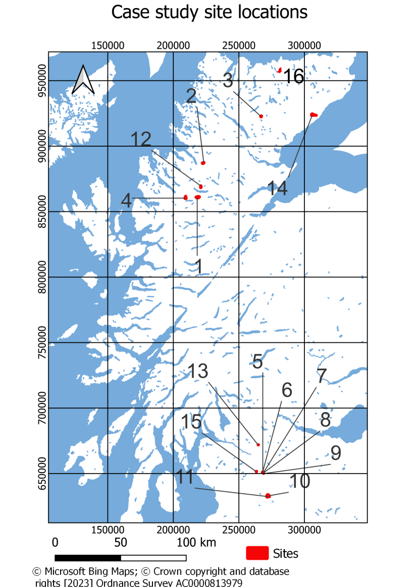
Figure 5: Locations of the case study sites, 1 Dos Mhucarain, 2 Carn Beag, 3 Ben Armine, 4 Carn na Garbh Lice, 5-9 Waukenwae Moss sites, 10,11 Tardoes Farm, 12 Coire Beag, 13 Lenzie Moss, 14 Strathy, 15 Langlands Moss, 16 Strathy North windfarm.
Click for a full description
Locations of case study sites, 1 Dos Mhucarain, 2 Carn Beag, 3 Ben Armine, 4 Carn na Garbh Lice, 5-9 Waukenwae Moss sites, 10,11 Tardoes Farm sites, 12 Coire Beag, 13 Lenzie Moss, 14 Strathy, 15 Langlands Moss, 16 Strathy North windfarm.
Lowland raised bogs
To summarise the condition and status of the three lowland raised bog sites, we chose a combination of condition and change. The target condition of the lowland raised bogs is clearly good, soft, and waterlogged and the trajectory of change status should be stable or positive. These attributes are presented using pie charts and descriptive summary statements (Figure 6).
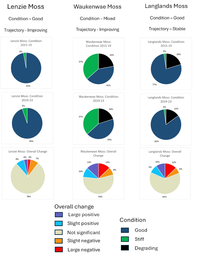
Figure 6: Pie charts and summary statements summarising the condition and overall trajectory of change for the three lowland raised bog sites.
Click for a full description
Pie charts and summary statements summarising the condition and trajectory of change for the three lowland raised bog sites. Lenzie Moss is predominantly good condition, less than 25% of the site shows significant change and on balance this change is positive. 43% of Waukenwae Moss is in good condition, 43% of the site shows significant change and on balance this change is positive. Langlands Moss is predominantly in good condition, 38% of the site shows significant change which is equally positive and negative.
Lenzie Moss
Lenzie Moss is a small, raised bog that has experienced extensive historic peat extraction. Observations and site characteristics are summarised in Table 2.
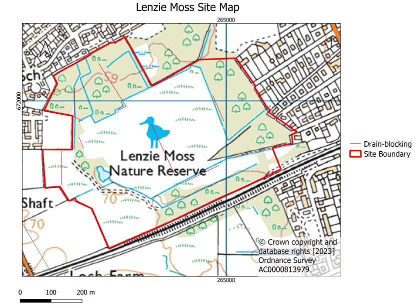
Figure 7: Lenzie Moss site map showing site boundary, areas and methods of restoration.
Click for a full description

Figure 8: Lenzie Moss maximum probability condition maps for the periods 2015-19 and 2019-23.
Click for a full description
Lenzie Moss maximum probability condition maps for the periods 2015-19 and 2019-23. Overall, the site is in good condition with stiff peat occurring around the margins. There is little change between periods of observation.
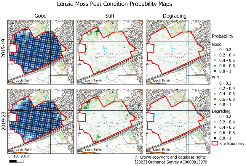
Figure 9: Lenzie Moss probability condition maps for the periods 2015-19 and 2019-23. Probabilities are shown for good, stiff and degrading classes.
Click for a full description
Lenzie Moss probability condition maps for the periods 2015-19 and 2019-23. Probabilities are shown for good, stiff and degrading classes. Overall, the site is in good condition with slightly stiffer margins. There is little change between periods of observation.
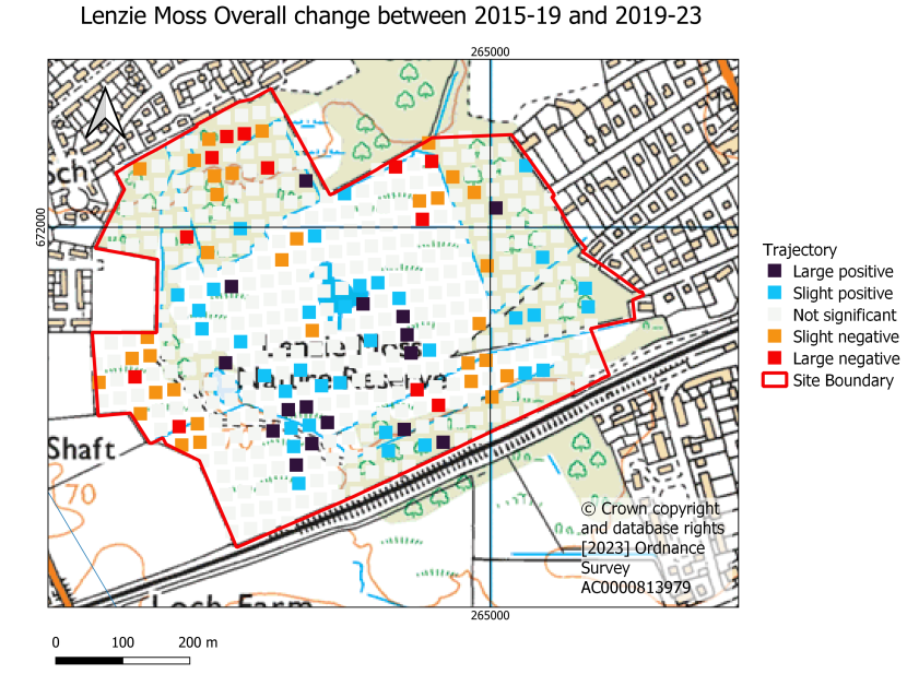
Figure 10: Lenzie Moss overall trajectory of change map based on comparison of the periods 2015-19 and 2019-23.
Click for a full description
Lenzie Moss overall trajectory of change map based on comparison of the periods 2015-19 and 2019-23. Most of the area shows no significant change. Most positive change occurs in the centre of the area and most negative change around the northern and western margin.
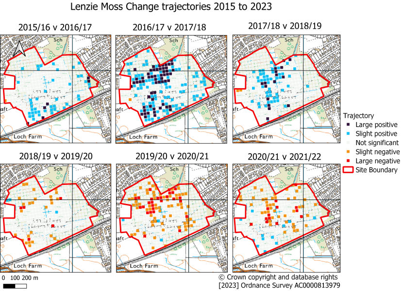
Figure 11: Lenzie Moss sequential annual trajectories of change from 2015 to 2023.
Click for a full description
Lenzie Moss sequential annual trajectories of change from 2015 to 2023. Most of the site shows no significant change. Where change occurs trajectories are generally improving from 2015/16 to 2018-19 and negative thereafter.
| Bog type | Landcover | Periods of restoration and methods used (Fig. 7) | Condition (Fig. 8 and 9) | Overall trajectory of change (Fig. 10) | Sequential change (Fig. 11) |
|---|---|---|---|---|---|
| Raised Bog | peat extraction, industrial | 2013-15, ditch blocking. 2016 ditch blocking 18/2/20 – 25/2/20, additional dams and scrub removal. | Good Probability of good condition declines along the W of the site | Predominantly stable Positive change in centre and negative around margins | 2015-19 positive or stable 2019-21 mainly stable or negative |
Interpretation
Overall, the site is in good condition following completion of the major restoration work in 2015 and 2016. Since 2019 the change trajectories indicate that the site is either stable or showing a local negative trajectory with negative trajectories occurring in the areas that showed a positive change from 2015-19. This may indicate that although in good condition the wetter areas on the site have gradually lost water from 2019-23. An overall negative change accompanied by a declining probability of good condition occurs along the western edge of the site and may indicate that this area, which based on topographic contours may be slightly more elevated, is more prone to hydrological stress and may be suffering from water table drawdown.
Waukenwae Moss
Waukenwae Moss is a complex of five sites containing raised bog. Observations and site characteristics are summarised in Table 3.

Figure 12: Waukenwae Moss site map showing site boundary, areas and methods of restoration. Discrete areas within the site are labelled 1,2,3,4 and 5 and are referred to in Table 3.
Click for a full description
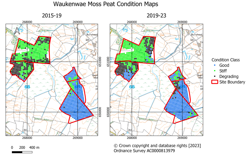
Figure 13: Waukenwae Moss maximum probability condition maps for the periods 2015-19 and 2019-23.
Click for a full description
Waukenwae Moss maximum probability condition maps for the periods 2015-19 and 2019-23. The southern sub-sites are in mainly in good condition. The northern sub-sites are predominantly stiff or degrading.

Figure 14: Waukenwae Moss probability condition maps for the periods 2015-19 and 2019-23. Probabilities are shown for good, stiff and degrading classes.
Click for a full description
Waukenwae Moss maximum probability condition maps for the periods 2015-19 and 2019-23. The southern sub-sites are in mainly in good condition. The northern sub-sites are predominantly stiff or degrading. The probability of good condition increases on the northern sites during 2019-23.
Change detection

Figure 15: Waukenwae Moss overall trajectory of change map based on comparison of the periods 2015-19 and 2019-23.
Click for a full description
Waukenwae Moss overall trajectory of change map based on comparison of the periods 2015-19 and 2019-23. Large positive change is most common in the northern site close to its southern boundary close to an area of drain blocking (Figure 12).

Figure 16: Waukenwae Moss sequential annual trajectories of change from 2015 to 2023.
Click for a full description
Waukenwae Moss sequential annual trajectories of change from 2015 to 2023. Mainly negative change is observed until 2018-19 followed by large positive change in the northern sub-site in 2019-20 then in the southeastern sub-sites in 2021-22.
| Site (Fig. 12) | Bog type | Landcover | Periods of restoration and methods used (Fig. 12) | Condition (Fig. 13 and 14) | Overall trajectory of change (Fig. 15) | Sequential change (Fig. 16) |
|---|---|---|---|---|---|---|
| Waukenwae Moss Area 1 | Raised Bog | intensive grassland | 28/10/19 – 11/11/19, Ditch blocking, peat and plastic dams, hag reprofiling, bunding | 2015-19 Predominantly stiff. Degrading on margins 2019-23 Predominantly stiff. Degrading on E margins Signs of improving condition in SE corner | Positive over area of ditch blocking Negative on eastern margin | Variable |
| Area 2 | Raised Bog | semi-natural, eroding | 28/10/19 – 11/11/19, ditch blocking, plastic dams | 2015-19 Mainly degrading to stiff. 2019-23 Good in south of area | Negative in centre and W, positive along N and E edge. | Positive response post 2019 close to areas of drain blocking on N and E boundaries. |
| Area 3 | Raised Bog | semi-natural, eroding | 28/10/19 – 11/11/19, Ditch blocking, peat dams, hag reprofiling, bunding | Predominantly good | Mixed, notably negative in N | Increasingly positive from 2019 onwards |
| Area 4 | Raised Bog | semi-natural, eroding | 28/10/19 – 11/11/19, Hag and peat bank reprofiling, bunding | 2015-29 Predominantly good, lesser area is stiff. 2019-23 Mixed stiff and good, minor area degrading. | Notably negative in S | Markedly positive in 2021/22 |
| Area 5 | Raised Bog | semi-natural, eroding | 28/10/19 – 11/11/19, Ditch blocking, peat dams, hag reprofiling, bunding | 2015-19 Predominantly good, stiff in NW corner. 2019-23 Predominantly good, degrading in NW corner. | Notably negative in W | Markedly positive in 2021/22 |
Interpretation
Overall, the two northern areas (boundary lies along the OS grid) are in a stiffer and more degrading condition than the three southern areas.
Area 1, as expected from dominant grassland vegetation, is in stiff condition but does display a positive response to restoration work. Areas 2, 3, 4 and 5 are all showing a stronger response to restoration which may reflect an initial less degraded state or a greater tendency to accumulate and store water. In this respect it is notable that areas 3,4 and 5 appear to be at slightly lower elevation.
Langlands Moss
Langlands Moss contains two areas of peat: an elevated lowland raised bog in the south of the site; and an area of peat in the north at the base of moderately steep slope that is more likely to have fen-like characteristics on account of groundwater discharge at the base of the slope. Observations and site characteristics are summarised in Table 4.
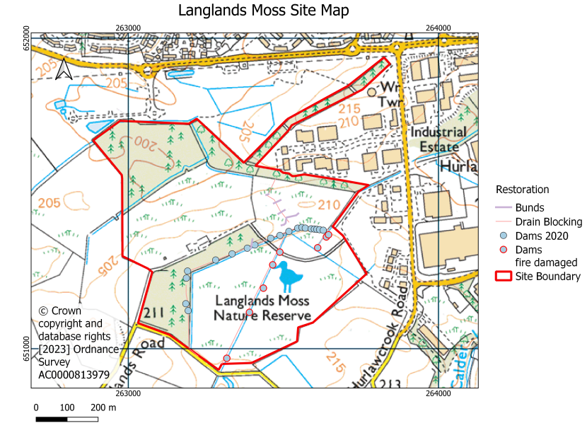
Figure 17: Langlands Moss site map showing site boundary, areas and methods of restoration.
Click for a full description

Figure 18: Langlands Moss maximum probability condition maps for the periods 2015-19 and 2019-23.
Click for a full description
Langlands Moss maximum probability condition maps for the periods 2015-19 and 2019-23. Degrading conditions occur in the centre of the southern site. There is little change between periods of observation.
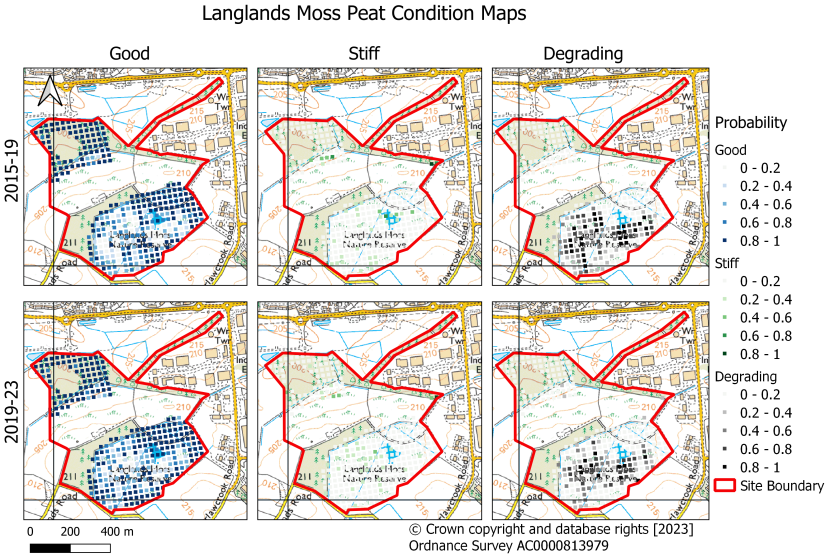
Figure 19: Langlands Moss probability condition maps for the periods 2015-19 and 2019-23. Probabilities are shown for good, stiff and degrading classes.
Click for a full description
Langlands Moss probability condition maps for the periods 2015-19 and 2019-23. Probabilities are shown for good, stiff and degrading classes. Degrading conditions occur in the centre of the southern site and good conditions in the northern site and around the periphery of the southern site. There is little change between periods of observation.

Figure 20. Langlands Moss overall trajectory of change map based on comparison of the periods 2015-19 and 2019-23.
Click for a full description
Langlands Moss overall trajectory of change map based on comparison of the periods 2015-19 and 2019-23. The site contains two areas of peat, the northernmost area shows negative change and the southernmost area shows positive change in the centre and negative change in the northeast that corresponds to an area badly affected by fire in 2017.
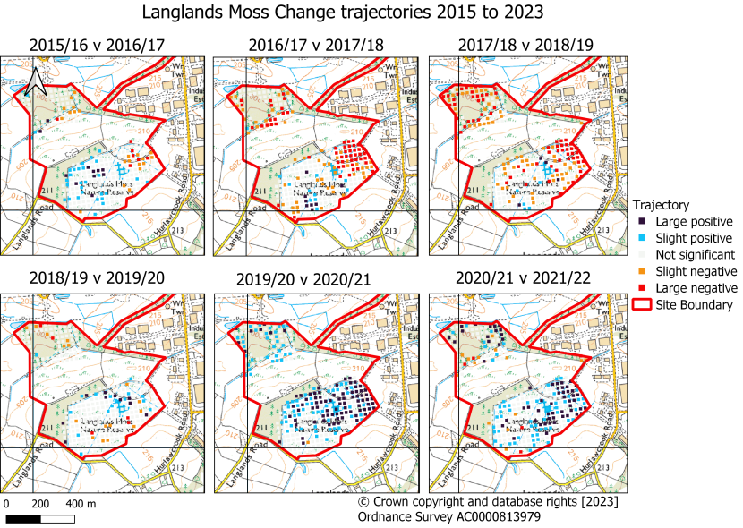
Figure 21: Langlands Moss sequential annual trajectories of change from 2015 to 2023.
Click for a full description
Langlands Moss sequential annual trajectories of change from 2015 to 2023. The site contains two areas of peat. Negative change in 2017-18 and 2018-19 in the northeast of the southern peat body corresponds to an area affected by fire in 2017. Positive change occurs in the southern peat body and slight positive change in the northern peat body in 2020-21 and 2021-22.
| Bog type | Landcover | Periods of restoration and methods used (Fig. 16) | Condition (Fig. 17 and 18) | Overall trajectory of change (Fig. 19) | Sequential change (Fig. 20) |
|---|---|---|---|---|---|
| Raised Bog | Semi-natural, eroding | 20/1/20 to 27/3/20, Ditch blocking, damming Felling, Jan-Feb 2020 | Mainly good, degrading locally, degrading in the centre of the S peat body. The probability of degrading peat in the S decreases between 2015-19 and 2019-23. | Negative in the N, positive in S centre, negative in NE of southern peat body. | 2015-19 Notable negative change in N peat body in 2018/19 Negative change in NE part of S peat body corresponds to area of fire in 2017. 2019-21 mainly positive post 2020 |
Interpretation
Two peat bodies occur within the site. The southern peat body experienced a fire along its northern edge (between the footpath and the edge of the peat) in 2017 and the area burnt displays a strong negative response following the fire in 2017/18, and 2018/19. Both northern and southern peat bodies, including the fire damaged area, display a strong positive response following restoration in early 2020. The south-central part of the southern peat body is locally degrading, and we suspect this may be the most elevated part of the body. Overall observations were consistent with observations made by D Large during a site visit in August 2023.
On optical imagery and during a site visit by D Large the northern peat body was observed to have been forested, partly covered in brash, with water present in open drains. The peat body also occurs at the base of a steep slope and therefore should be in an area of natural seepage. It seems probable that the winter swelling in this setting should be interpreted as a direct indicator of the potential of the area to store water and the potential for ecological restoration.
Blanket bog sites
When interpreting condition and change over areas of eroded peat containing gullies and hags, the InSAR signal from an area of 20 x 20 m may consist of a mixed contribution from hags, gully sides, the bases of gullies and the areas of peatland between the gullies. Therefore, the following must be considered:
- Extensive and prolonged erosion leads to stiff consolidated peat (Marshall et al., 2022). It should therefore be expected that many of these areas will be dominated by stiff peat.
- Gullies will vary in character:
- If they are actively losing material, they will be subsiding and hence classed as actively degrading.
- If they are down to bare mineral soil, they will be stiff.
- If the gullies are stable and wet and variably vegetated, they will be in good condition, as observed in places in Cairnsmore (Bradley et al., 2025) and extensively on Knockfin Heights (Marshall et al., 2022).
- Where erosion is most active either on account of incision, formation of peat pipes, or net removal of peat by wind or water, then subsidence will occur, and the areas will be classed as degrading.
- On steep ground, erosion by mass movement (landslide or creep) will generate a vertical component of motion that will be recorded as subsidence in the InSAR signal and hence classified as degrading.
- Intervention in these areas is often by hag reprofiling which involves heavy excavators tasked with reducing the slope of the hags and revegetating with turf borrowed from nearby. The presence of heavy machinery will rapidly increase consolidation of the peat, which will lead to stiffening. It will also reduce the area of the gullies and shift the balance of the InSAR signal in favour of stiff peat. Subsequent recovery, where water is retained, is likely to be initially marked by swelling rather than establishment of a dynamic surface motion. Initially this will be most apparent by measures of change detection.
When summarising the status of the blanket bog sites, the key issues are:
- Much of the restoration work was done relatively late (2020-21) in the period of observation.
- There is a fundamental question as to the aim of restoration. This is likely to vary depending on level of erosion, peat depth and slope angles. Flatter areas will be more suited to rewetting with a target state of soft wet good conditions and steeper areas will be more stable in a stiff condition.
- Many of the sites contain extensive eroded upland peat that is now in stiff condition and therefore slow to respond to restoration.
- Signals from areas of peat hags and gullies may be a mixture of the response from the gully or hag and adjacent intact peatland.
Due to the late dates of restoration, we chose measures of overall change to summarise the status of the sites. This method has the advantage of being based on the comparison of two 4-year periods and encapsulating the entire dataset.
There are numerous alternative means of summarising. For example, a measure of the area undergoing positive change each year, or at the end of a period of interest could be useful but somewhat weather prone. A reduction in the area undergoing degradation would also be appropriate but only if the site still has areas capable of displaying rapid subsidence.
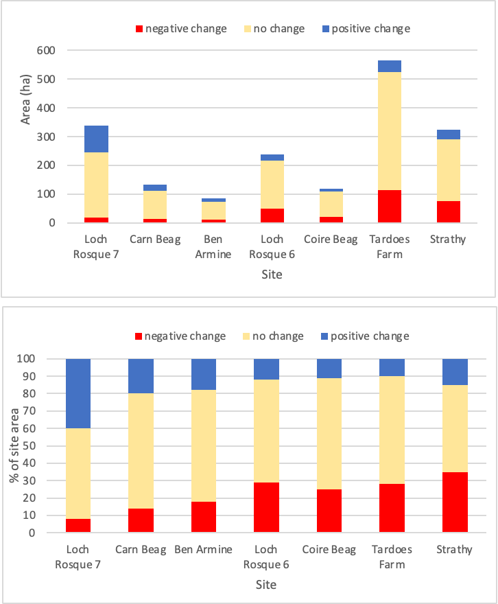
Figure 22: Comparison of trajectories of change in the blanket bog case study sites expressed on an area basis (A) and a percentage basis (B).
Click for a full description
Comparison of trajectories of change in the blanket bog case study sites expressed on an area basis (A) and a percentage basis (B). Case studies are Lochrosque 7, Carn Beag, Ben Armine, Lochrosque 6, Coire Beag, Tardoes Farm and Strathy. Calculations are based on the number of pixels contained within a site and the area of the site. On an area and percentage basis Lochrosque 7 is performing best with positive change greatly exceeding negative change. Steeper sites at Lochrosque 6, Coire Beag and Tardoes Farm perform least well with negative change exceeding positive change.
The summary indicates that the best performing of the upland eroded sites is Lochrosque Phase 7 in which about 40% of the site is displaying positive change. This is followed by Carn Beag and Ben Armine with about 20% positive change, then Lochrosque Phase 6, Coire Beag and Tardoes Farm with about 10% positive change each. Strathy is somewhat different, being lower in altitude and dominated by drains with comparatively few areas of erosion. The most striking feature that may explain the response of the eroded upland sites is gradient, which in essence determines the ability of the site to retain water and re-wet. Lochrosque Phase 7 has large areas of low gradient terrain (<2°), then Carn Beag and Ben Armine having somewhat steeper gradients (2-3°) and Lochrosque Phase 6, Coire Beag and Tardoes Farm have extensive areas of steep slopes (>5°).
Ben Armine
Overall, the site is eroded and gently sloping with a SW aspect. Minor watersheds draining SE and W occur at altitudes of 445 m and 458 m, respectively. The most intensive erosion occurs on these watersheds. Observations and site characteristics are summarised in Table 5.
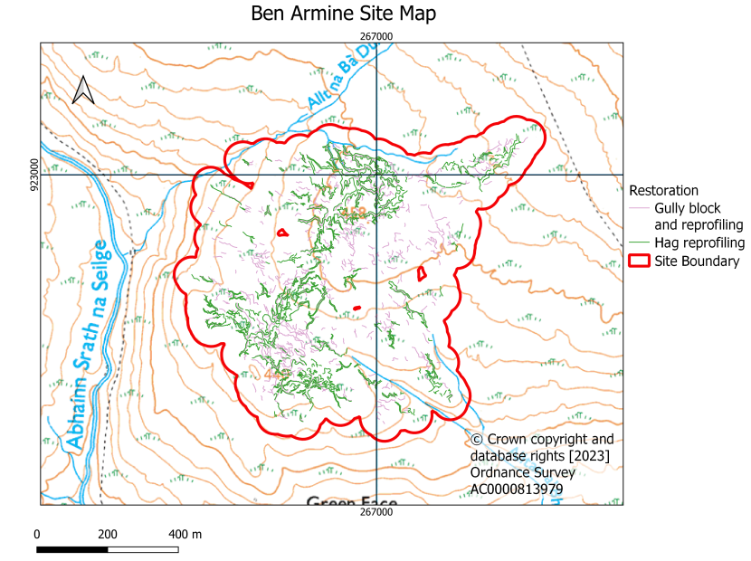
Figure 23: Ben Armine site map showing site boundary, areas and methods of restoration.
Click for a full description
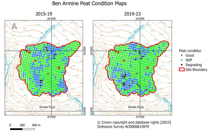
Figure 24: Ben Armine maximum probability condition maps for the periods 2015-19 and 2019-23.
Click for a full description
Ben Armine probability condition maps for the periods 2015-19 and 2019-23. Good condition occurs in a band through the centre of the site, stiff condition occurs to the east and west of the site. The most obvious change during the period of observation is stiffening in the centre of the site and an increase in the area in good condition in the southwest of the site.

Figure 25: Ben Armine probability condition maps for the periods 2015-19 and 2019-23. Probabilities are shown for good, stiff and degrading classes.
Click for a full description
Ben Armine probability condition maps for the periods 2015-19 and 2019-23. Good condition occurs in a band through the centre of the site, stiffer conditions occur to the east and west of the site and degrading condition occurs locally on the upslope extensions of natural drainage lines. The most obvious change during the period of observation is stiffening in the centre of the site and an increase in the area in good condition in the southwest of the site.

Figure 26: Ben Armine overall trajectory of change map based on comparison of the periods 2015-19 and 2019-23.
Click for a full description
Ben Armine overall trajectory of change map based on comparison of the periods 2015-19 and 2019-23. Most of the site shows no significant change. Scattered positive change is more prevalent in the east of the site. Scattered negative change is more prevalent in the west of the site.
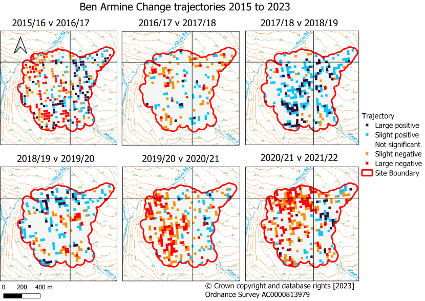
Figure 27: Ben Armine sequential annual trajectories of change from 2015 to 2023.
Click for a full description
Ben Armine sequential annual trajectories of change from 2015 to 2023. Marked positive change occurs across the site in 2018-19 and marked negative change occurs in the west and north of the site in 2020-21 and 2021-22.
| Bog type | Landcover | Periods of restoration and methods used (Fig. 23) | Condition (Fig. 24 and 25) | Overall trajectory of change (Fig. 26) | Sequential change (Fig. 27) |
|---|---|---|---|---|---|
| Blanket Bog | Semi-natural, eroding | 12/11/19 to 14/12/20 Bunding, damming, hag reprofiling | Mainly stiff with distinct patches of good condition Probability maps show stiffening in the central part of the site and expansion of improving conditions in the N and particularly the S of the site. Degrading areas are mainly associated with the upslope extensions of natural drainage lines | Mainly stable, patchy negative change is more common in W half of site and positive change in the eastern part of the site | 2015-19 A notable positive change occurs in 2018/19 2019-21 Some positive change in 2019/20, followed by mainly negative change in the W half of the site |
Interpretation
Stiff conditions are predominantly associated with areas of minimal intervention or areas of predominantly hag reprofiling. Degrading conditions on the probability maps are associated with the upper extension of natural drainage lines and this may indicate incision and headward extension of the natural drainage system. Areas in good condition prior to 2019 are somewhat more localised and probably indicate areas where drainage was less effective, or peat was prone to natural recovery within gullies. Areas in good condition post 2019 are associated with areas of intense restoration work, on flatter ground on natural watersheds and are therefore more likely to retain water. An area with a greater probability of being good condition expands notably in the SW of the site post-restoration and this may indicate that this downslope area is rewetting more effectively than its upslope counterpart. It should be noted that very few areas have a high probability of being in good condition.
Positive change occurs in response to restoration work in 2019 and 2020. Thereafter the eastern half of the site appears to be relatively stable and prone to slight positive change and the western half more prone to negative change.
Carn Beag
The site is extensively eroded with gullies and hags. Most of the site slopes gently W with and area of flatter ground and possibly eroded pool systems on a watershed in the NE. Observations and site characteristics are summarised in Table 6.
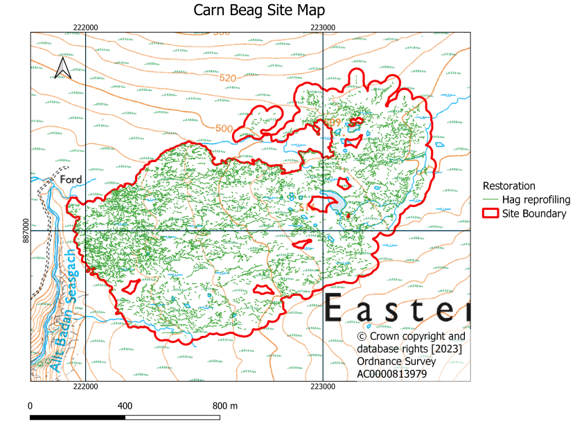
Figure 28: Carn Beag site map showing site boundary, areas and methods of restoration.
Click for a full description
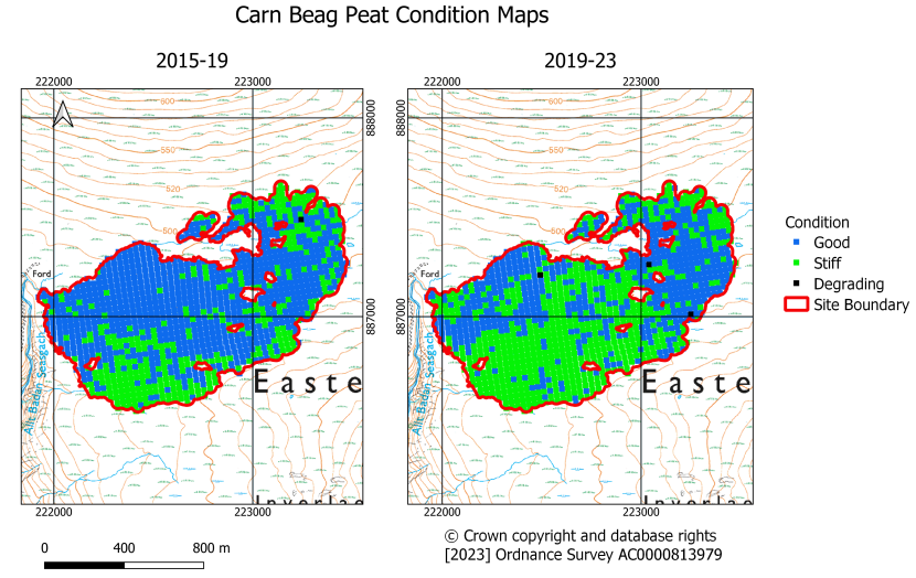
Figure 29: Carn Beag maximum probability condition maps for the periods 2015-19 and 2019-23.
Click for a full description
Carn Beag maximum probability condition maps for the periods 2015-19 and 2019-23. The site is predominantly in stiff or good condition and the major change is a stiffening of the site during 2019-23.
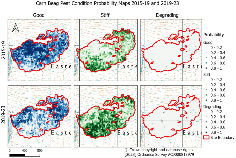
Figure 30: Carn Beag probability condition maps for the periods 2015-19 and 2019-23. Probabilities are shown for good, stiff and degrading classes.
Click for a full description
Carn Beag probability condition maps for the periods 2015-19 and 2019-23. The site is predominantly in stiff or good condition and the major change is a stiffening of the central part of the site during 2019-23. Stiffer areas in the south and central part of the site correspond to areas with less intensive restoration (Figure 28).

Figure 31: Carn Beag overall trajectory of change map based on comparison of the periods 2015-19 and 2019-23.
Click for a full description
Carn Beag overall trajectory of change map based on comparison of the periods 2015-19 and 2019-23. Scattered positive change is more prevalent in the east and west of the site and scattered negative change more prevalent in the centre of the site.
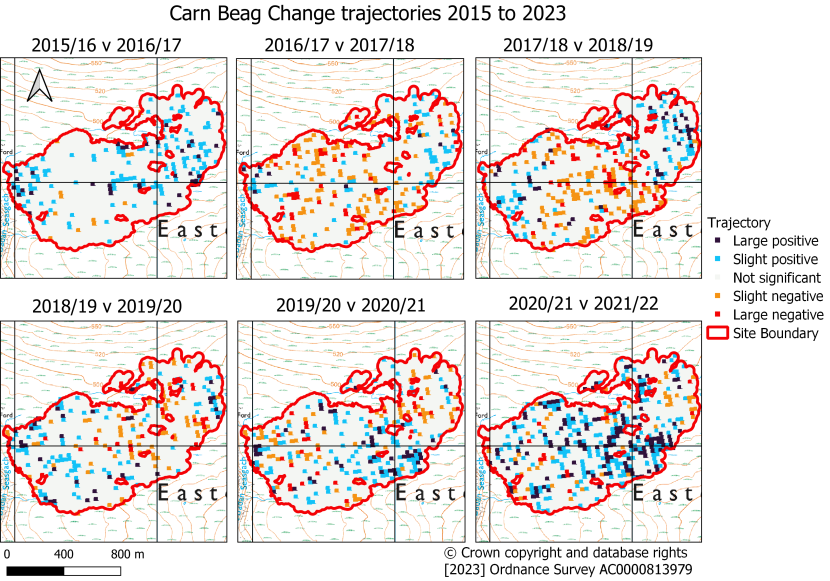
Figure 32: Carn Beag sequential annual trajectories of change from 2015 to 2023.
Click for a full description
Carn Beag sequential annual trajectories of change from 2015 to 2023. The most distinct feature is notable positive change in 2021-22.
| Bog type | Landcover | Periods of restoration and methods used (Fig. 28) | Condition (Fig. 29 and 30) | Overall trajectory of change (Fig. 31) | Sequential change (Fig. 32) |
|---|---|---|---|---|---|
| Blanket Bog | Semi-natural, eroding | 2/03/21– 23/07/21 Hag reprofiling | 2015-19 Mainly good 2019-21 Mainly stiff Areas with particularly high probability of being in good condition occur in N and NE of site | Variable positive and negative change across the site | Extensive positive change in 2021/22 |
Interpretation
The site is extensively eroded. A general stiffening of the site in 2019-23 is notable probably in response to restoration activities. Good condition is prevalent across the N and NE of the site in 2015-19 and probably reflects the low gradient and water retentiveness of the gullies. The area of good condition contracts in 2019-23 potentially in response to reprofiling work, contraction of the area of gullies and stiffening of the site. A positive change is notable in 2021/22 and may reflect a response to the restoration work.
Carn na Garbh Lice: Lochrosque Phase 6
The site is an extensively eroded area of peat on the relatively steep NE and SE slopes of Carn na Garbh Lice. Flattest ground is found on the col 1 km east of the summit. Observations and site characteristics are summarised in Table 7.
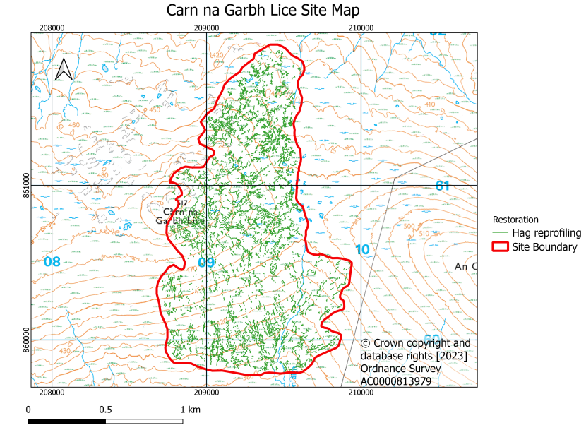
Figure 33: Carn na Garbh Lice site map showing site boundary, areas and methods of restoration.
Click for a full description
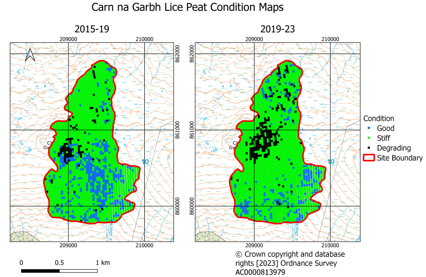
Figure 34: Carn na Garbh Lice maximum probability condition maps for the periods 2015-19 and 2019-23.
Click for a full description
Carn na Garbh Lice probability condition maps for the periods 2015-19 and 2019-23. The site is predominantly stiff. In 2019-23 an increase in good condition is observed in the south of the site whereas in the north of the site the areas in degrading condition increases.
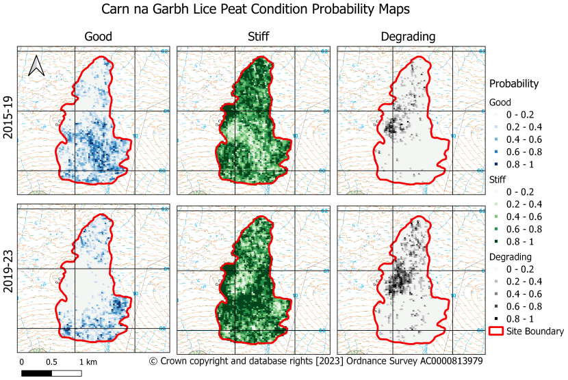
Figure 35: Carn na Garbh Lice probability condition maps for the periods 2015-19 and 2019-23. Probabilities are shown for good, stiff and degrading classes.
Click for a full description
Carn na Garbh Lice probability condition maps for the periods 2015-19 and 2019-23. The site is predominantly stiff. In 2019-23 an increase in the probability of being in good condition is observed in the south of the site whereas in the north of the site the probability of being in degrading condition increases.

Figure 36: Carn na Garbh Lice overall trajectory of change map based on comparison of the periods 2015-19 and 2019-23.
Click for a full description
Carn na Garbh Lice overall trajectory of change map based on comparison of the periods 2015-19 and 2019-23. Scattered areas of negative change are more extensive than areas of positive change with more negative change in the north of the site.

Figure 37: Carn na Garbh Lice sequential annual trajectories of change
Click for a full description
Carn na Garbh Lice sequential annual trajectories of change from 2015 to 2023. The most distinct feature is notable negative change in 2021-22.
| Bog type | Landcover | Periods of restoration and methods used (Fig. 33) | Condition (Fig. 34 and 35) | Overall trajectory of change (Fig. 36) | Sequential change (Fig. 37) |
|---|---|---|---|---|---|
| Blanket Bog | Semi-natural, eroding | 14/12/20– 4/08/2021 Hag reprofiling | Mainly stiff. Degrading in centre and N of site on steep E slopes of Carn na Garbh Lice. Peat in good condition occurs predominantly in the S of the site. Probability maps show the site becomes increasingly more degraded on the steeper slopes east of Carn na Garbh Lice and in the N of the site | No clear pattern | Distinct negative change in 2021/22 in N of area |
Interpretation
As expected on such a steep site the condition is predominantly stiff. The most notable change comparing 2015-19 to 2019-23 is the increase in stiff and degrading conditions. Degrading conditions have the highest probability on the steepest ground raising the question as to whether the restoration work in these areas may have caused more subsidence or mass movement. The probability that peat is in good condition is not particularly high with very few pixels in the top two probability classes. Areas with a high probability of being in good condition are predominantly found close to natural drainage lines in the south of the site. In terms of change the only distinct signal is a strong negative trend in 2021/22 in the north of the site which could be a direct response to restoration activities that ended in August 2021.
Dos Mhucarain: Lochrosque Phase 7
The site is predominantly within the upper catchment of the Allt Mor. Upper parts of the catchment have gentle slopes and are intensively eroded. Surrounding slopes are steeper and included areas of drains, notably upslope to the west and downslope to the east. Observations and site characteristics are summarised in Table 8.
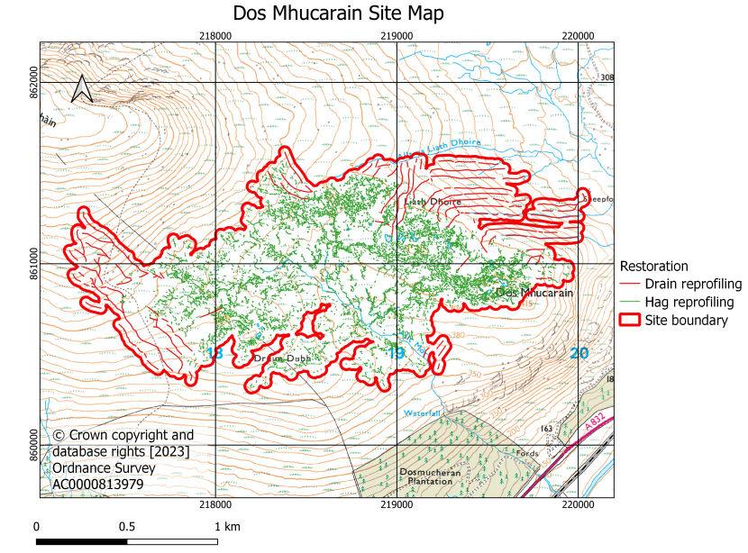
Figure 38: Dos Mhucarain site map showing site boundary, areas and methods of restoration.
Click for a full description
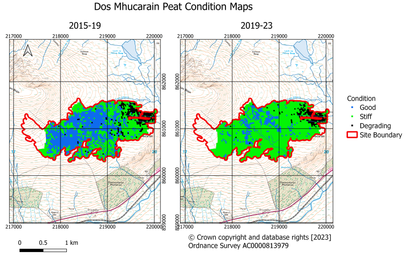
Figure 39: Dos Mhucarain maximum probability condition maps for the periods 2015-19 and 2019-23.
Click for a full description
Dos Mhucarain maximum probability condition maps for the periods 2015-19 and 2019-23. Overall, the site is in good condition during 2015-19 and in stiffer condition from 2019-23. Degrading conditions occur on the eastern edge of the site and the area in degrading condition reduces in 2019-23.

Figure 40: Dos Mhucarain probability condition maps for the periods 2015-19 and 2019-23. Probabilities are shown for good, stiff and degrading classes.
Click for a full description
Dos Mhucarain probability condition maps for the periods 2015-19 and 2019-23. The site has higher probabilities of being in good condition during 2015-19 and of being is stiffer condition from 2019-23. Degrading conditions occur on the eastern edge of the site and the area in degrading condition reduces in 2019-23.
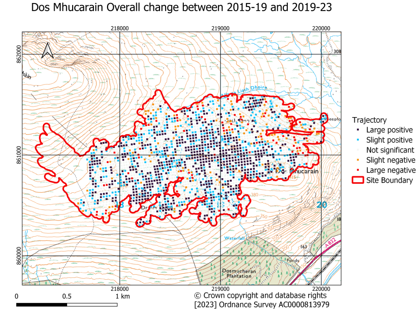
Figure 41: Dos Mhucarain overall trajectory of change map based on comparison of the periods 2015-19 and 2019-23.
Click for a full description
Dos Mhucarain overall trajectory of change map based on comparison of the periods 2015-19 and 2019-23. Extensive areas of large positive change occur in the centre of the site.
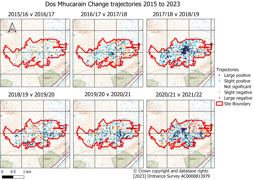
Figure 42: Dos Mhucarain sequential annual trajectories of change from 2015 to 2023.
Click for a full description
Dos Mhucarain sequential annual trajectories of change from 2015 to 2023. Extensive positive change occurs in 2018-19 and in 2021-22.
| Bog type | Landcover | Periods of restoration and methods used (Fig. 38) | Condition (Fig. 39 and 40) | Overall trajectory of change (Fig, 41) | Sequential change (Fig. 42) |
|---|---|---|---|---|---|
| Blanket bog | Semi-natural, eroding | 19/10/20 - 23/03/21 Drain blocking, drain reprofiling, hag reprofiling. | 2015-19 Mainly good in centre of site associated with flatter areas, breaks in slope and upslope extensions of natural drainage lines, degrading on steeper slopes in E of site associated with areas of drains, other margins stiff. 2019-23 Stiffer throughout, good conditions confined to arcuate area at head of Allt Mor, reduced area of degrading peat on E margin | Mainly positive within the gently sloping eroded source region of the Allt Mor. | 2015-19 Notable positive change in 2018/19 corresponds to area of the most continuous and least eroded peat on the site. 2019-21 notable positive change across central and S of site in 2021/22 |
Interpretation
The most striking change in the condition of the site is a marked stiffening of the peat in the 2019-23, with a reduction in the area of peat in good and degrading condition. Peat in good condition remains associated with flatter ground and the upslope extension of natural drainage lines, presumably in areas of seepage. A probable reason for stiffening is the restoration work and associated compaction by excavators, evidence of this being the extensive vehicle tracks observed on top of the hags in some optical images. The reduction in the extent of degrading peat in the east occurs in areas that have experienced drain blocking.
The marked positive change in 2018/19 in the centre of the site may indicate recovery of an area of peat in good condition on the site after the spring drought of 2018. Given that the restoration was only completed in early 2021, the overall change map that extends the period of measure to early 2023 is the map most likely to capture change in response to this restoration. This map shows extensive positive change.
A combination of stiffening and positive change is indicative of swelling of the peat without the development of notable seasonal oscillations.
Coire Beag
The area is a steep south facing corrie drained by the Allt a Choire Bhig. Peat is characterised by intensive erosion. The southern part of the site has historically been drained but drain reprofiling has been undertaken in recent years. Observations and site characteristics are summarised in Table 9.

Figure 43: Coire Beag site map showing site boundary, areas and methods of restoration.
Click for a full description
Coire Beag site map.
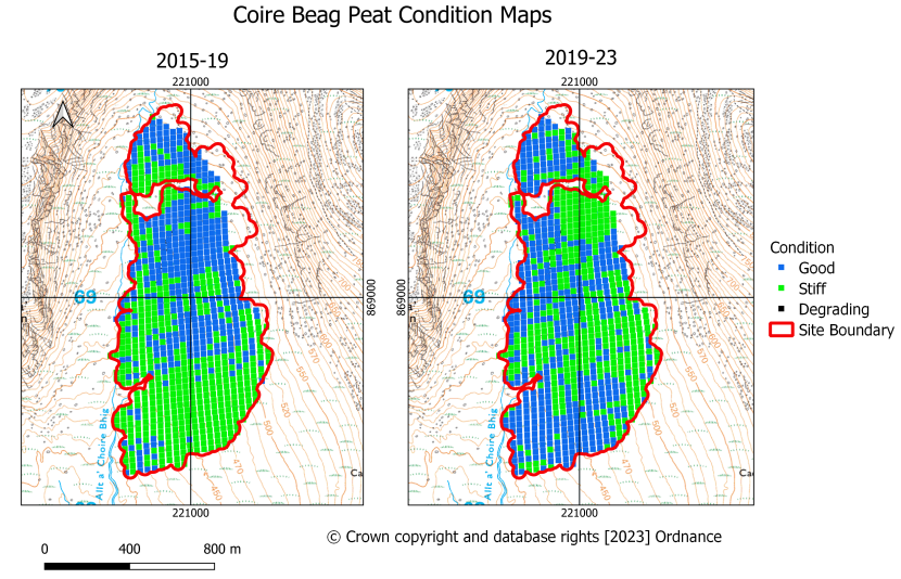
Figure 44: Coire Beag maximum probability condition maps for the periods 2015-19 and 2019-23.
Click for a full description
Coire Beag maximum probability condition maps for the periods 2015-19 and 2019-23. From 2015-19 the northern and western part of the is in good condition and the southern part of the site in stiff condition. This situation reverses in 2019-23.
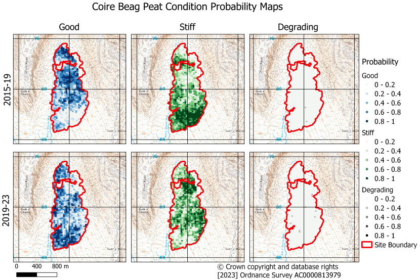
Figure 45: Coire Beag probability condition maps for the periods 2015-19 and 2019-23. Probabilities are shown for good, stiff and degrading classes.
Click for a full description
Coire Beag probability condition maps for the periods 2015-19 and 2019-23. From 2015-19 the northern part of the site has a higher probability of being in good condition than the southern part of the site, which is in stiff condition. This situation reverses in 2019-23.
Change detection
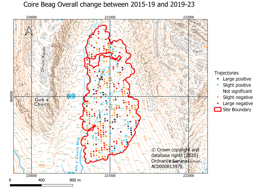
Figure 46: Coire Beag overall trajectory of change map based on comparison of the periods 2015-19 and 2019-23.
Click for a full description
Coire Beag overall trajectory of change map based on comparison of the periods 2015-19 and 2019-23. Most of the site displays no significant change with a few scattered patches of large negative change in the south and very few areas showing large positive change.

Figure 47: Coire Beag sequential annual trajectories of change from 2015 to 2023.
Click for a full description
Coire Beag sequential annual trajectories of change from 2015 to 2023. Areas of extensive large positive change occur in the northern half of the site in 2021-22. Areas showing large negative change are most persistent in the south and north of the site in 2019-20 and 2020-21.
| Bog type | Landcover | Periods of restoration and methods used (Fig. 43) | Condition (Fig 44 and 45) | Overall trajectory of change (Fig. 46) | Sequential change (Fig. 47) |
|---|---|---|---|---|---|
| Blanket bog | Semi-natural, eroding | 13/01/20– 01/03/21 Ditch blocking, ditch reprofiling, bunding. Hag reprofiling, hag block | 2015-19 Mainly good in N and stiff in S. 2019-23 Large area in good condition in S and stiffer in N | Mainly stable to negative | 2015-19 Somewhat negative in 2017/18 and positive in 2018/19 2019-21 negative in N, E and S of site in 2019/20 and 2020/21. Marked positive change in N of site in 2021/22 |
Interpretation
Overall pattern of condition and change indicates a general stiffening in the north of the site and increase in water storage and improving condition in the south of the site. The overall sense is that the focus of water storage appears to have moved downslope from the areas of natural seepage, and this may relate to the restoration work generating more storage in the south and west of the site via drain reprofiling and more consolidation via hag reprofiling in the north and east.
It may also be that overall retention of the water in the corrie has resulted in more seasonal swelling of the peat downslope (hence a shift from stiff to good condition). The overall change map does not display a positive response in the south, as may be expected from the general trend from stiff to good condition; this may be due to the long-term trajectory not being impacted greatly as the ground is relatively steep and the boulder icon in the Ordnance Survey mapping suggests the peat layer is relatively thin. Unfortunately, peat depths for this site are not reported.
Strathy
The area contains four separate sites all of which have been drained with no areas of extensive erosion identified. Most of the sites are gently sloping minor watersheds between tributaries of the Langwell Water. Steep ground occurs towards the northern edge of the two westernmost sites. Observations and site characteristics are summarised in Table 10.
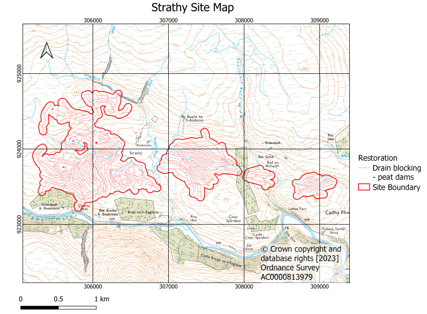
Figure 48: Strathy site map showing site boundary, areas and methods of restoration.
Click for a full description

Figure 49: Strathy maximum probability condition maps for the periods 2015-19 and 2019-23.
Click for a full description
Strathy maximum probability condition maps for the periods 2015-19 and 2019-23. The site consists of four sub-sites. During 2015-23 the smaller easternmost site is predominantly in good condition and the remaining sites are in a predominantly stiff condition. From 2019-23 the area in good and degrading condition increases markedly in the two western sub-sites. The other sites remain little changed. Degrading conditions are associated with steeper ground in the northern part of the two western sub-sites.
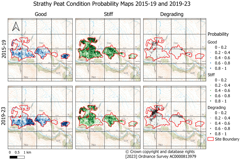
Figure 50: Strathy probability condition maps for the periods 2015-19 and 2019-23. Probabilities are shown for good, stiff and degrading classes.
Click for a full description
Strathy probability condition maps for the periods 2015-19 and 2019-23. Comparing the two periods the main change is an increase in the areas with higher probabilities of being in good or degrading condition and a reduction in the areas in stiff condition particularly in the western sites. Probabilities of degrading condition increase most notably on steeper ground in the westernmost subsite.
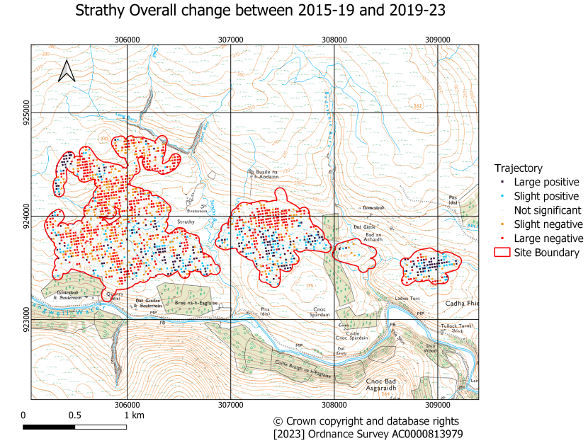
Figure 51: Strathy overall trajectory of change map based on comparison of the periods 2015-19 and 2019-23.
Click for a full description
Strathy overall trajectory of change map based on comparison of the periods 2015-19 and 2019-23. Negative change is extensive in the northern parts of the two western sub-sites. Positive change is not in the southeast of the and south of the two western sub-sites and in the centre of the eastern sub-site.
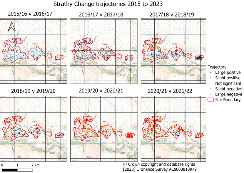
Figure 52: Strathy sequential annual trajectories of change from 2015 to 2023.
Click for a full description
Strathy sequential annual trajectories of change from 2015 to 2023. Positive change is most notable in 2018-19 and 2019-20 particularly in the eastern sub-site. Negative change is most prominent in 2020-21 and 2021-22 particularly in the northern half of the western sub-site.
| Bog type | Landcover | Periods of restoration and methods used (Fig. 48) | Condition (Fig. 49 and 50) | Overall trajectory of change (Fig 51) | Sequential change (Fig. 52) |
|---|---|---|---|---|---|
| Blanket bog | Semi-natural, eroding | 06/01/20– 04/02/20 Drain blocking, drain reprofiling. | 2015-19 E area mainly good. W areas mainly stiff. 2019-23 E area mainly good. W areas have a greater extent of good condition in S and of degraded condition in N. | Positive in the centre of the E area. Negative in the north of the two westernmost areas and positive in the south and southeast of these areas. | 2015-19 Easternmost area displays marked positive change in 2018/19 2019-21 Easternmost area displays marked negative change in 2020/21 Easternmost and the two western areas display positive change in areas of positive change that are similar to those observed in the overall change map. |
Interpretation
The site provides an interesting case study with respect to restoration response and landscape position. Positive responses to restoration occur on flatter areas that will better accumulate water. The most successful of these is the eastern area which, displays a marked positive response in 2018/19 following the 2018 drought and (presumably on account of near surface wetness) also displays a strong negative response to the locally dry early summer of 2020. Overall, the amount peat in good condition increases in the period 2019-23 post restoration and the areas of notable improvement correspond to the areas of positive change on the overall change map. The area of degrading peat also increases, particularly in the westernmost area, and this increase is associated with steeper ground. This raises the question as to why restoration work on the steeper ground appears to have destabilised the peat. Possible explanations include mass movement or increased discharge and erosion through peat pipes, both of which could occur on account of increased wetness.
Tardoes Farm
The site is complex and steep with areas of drainage and erosion. Eroded peat generally occurs on the upper slopes and the col between Priesthill Height and Starpet Rig. Observations and site characteristics are summarised in Table 11.

Figure 53: Tardoes Farm site map showing site boundary, areas and methods of restoration.
Click for a full description

Figure 54: Tardoes Farm maximum probability condition maps for the periods 2015-19 and 2019-23.
Click for a full description
Tardoes Farm maximum probability condition maps for the periods 2015-19 and 2019-23. Degrading conditions occur throughout. Good conditions occur in the north and centre of the site and stiff conditions occur around the periphery. The main change in 2019-23 is an increase in degrading conditions on steeper ground in the eastern part of the site.
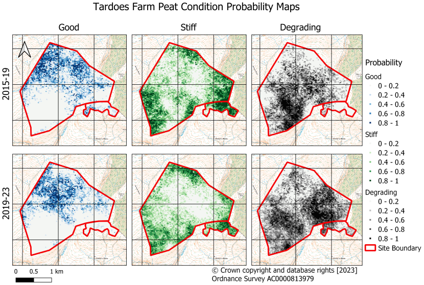
Figure 55: Tardoes Farm probability condition maps for the periods 2015-19 and 2019-23. Probabilities are shown for good, stiff and degrading classes.
Click for a full description
Tardoes Farm maximum probability condition maps for the periods 2015-19 and 2019-23. The southern sub-sites are in mainly in good condition. Moderate to high probabilities of degrading conditions occur throughout. Higher probabilities of good condition occur in the north of the site and higher probabilities of stiff conditions occur around the periphery. The main change in 2019-23 is an increasing probability of degrading conditions on steeper ground in the eastern part of the site.
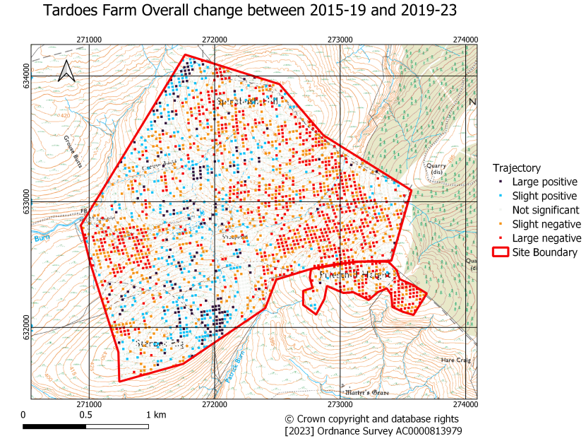
Figure 56: Tardoes Farm overall trajectory of change map based on comparison of the periods 2015-19 and 2019-23.
Click for a full description
Tardoes Farm overall trajectory of change map based on comparison of the periods 2015-19 and 2019-23. Negative change is widespread in the eastern half of the site and close to the western edge. Slight positive change occurs in the centre of the site.
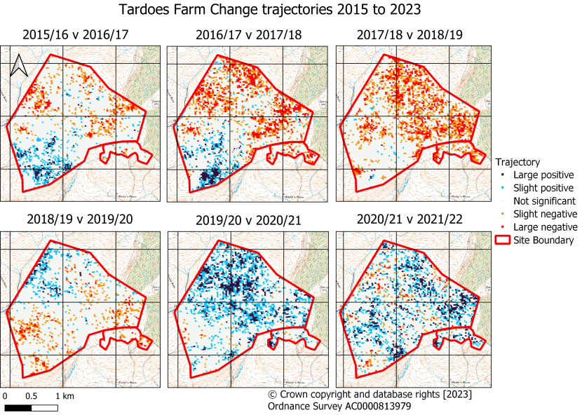
Figure 57: Tardoes Farm sequential annual trajectories of change from 2015 to 2023.
Click for a full description
Tardoes Farm sequential annual trajectories of change from 2015 to 2023. Negative change in the northern half of the site is widespread in 2017-18 and 2018-19. Extensive positive change occurs in 2020-21 and 2021-22 particularly in the north and east of the site.
| Bog type | Landcover | Periods of restoration and methods used (Fig. 52) | Condition (Fig. 53 and 54) | Overall trajectory of change (Fig. 55) | Sequential change (Fig. 56) |
|---|---|---|---|---|---|
| Blanket bog | Not provided | 09/09/19– 27/3/20, Ditch blocking, ditch reprofiling, hag reprofiling | 2015-19 Good condition in centre and N. However very few pixels have a high probability of being in good condition Degrading conditions are scattered throughout but more in the south associated with areas of drains and steep ground on Starpet Rig. Stiff peat mainly occurs on steep ground and hill tops. 2019-21 Similar to above but with an increase in the area of degrading peat on the steep slopes of Priesthill Height and Spirebush Hill. | Negative on the steep slopes of Spirebush Hill and Priest Hill Height positive in centre and south | 2015-19 Negative change in north and east and locally positive in the south on Starpet Rig 2019-21 Marked positive change across site in 2020/21 and scattered positive change across site in 2021/22 |
Interpretation
The very few pixels with a high probability of being in good condition are mainly found in the northern part of the site north of the Leaze Burn, on what are slightly gentler slopes. Hilltops as expected are generally stiff (Priesthill Height, Spirebush Hill) or degrading (Starpet Rig), probably on account of having thin peat. The summit of Starpet Rig also shows a positive trajectory, with both observations being consistent with this area containing deeper peat than the other hill tops. Although much of the area displays evidence of a positive trajectory post-restoration, the quantity of degrading peat also increases particularly on the steep slopes of Priesthill Height. The increase in degrading peat in this area could indicate that rewetting as a result of drain blocking is leading to either increased erosion, possibly via peat pipes or mass movement.
Windfarm
Observations and site characteristics are summarised in Table 12.
Strathy North
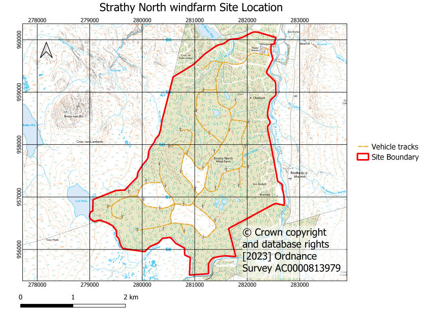
Figure 58: Strathy North Windfarm site map showing site boundary, areas and methods of restoration.
Click for a full description

Figure 59: Strathy North Windfarm maximum probability condition maps for the periods 2015-19 and 2019-23. Areas A, B and C show a transition from degrading to better condition which is interpreted as evidence of ponding of water upslope from tracks.
Click for a full description
Strathy North Windfarm maximum probability condition maps for the periods 2015-19 and 2019-23. Degrading conditions are common in the centre and southwest of the site. The main change in 2019-23 is stiffening along the road network, a decrease of the area in degrading condition and an increase in the area in good condition. Areas labelled A, B and C are areas that show a transition from degrading to better condition which is interpreted as evidence of ponding of water upslope from vehicle tracks.
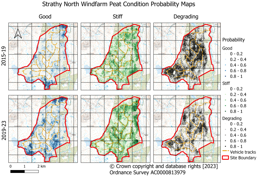
Figure 60: Strathy North Windfarm probability condition maps for the periods 2015-19 and 2019-23. Probabilities are shown for good, stiff and degrading classes.
Click for a full description
Strathy North Windfarm probability condition maps for the periods 2015-19 and 2019-23. Higher probabilities of stiff peat occur on steeper ground and track the roads on the site. Higher probabilities of degrading and good conditions occur in discrete road bounded areas throughout. The main change over time is a stiffening of the roads and an increase in the area with a probability of good condition and reduction in the area in degrading condition.
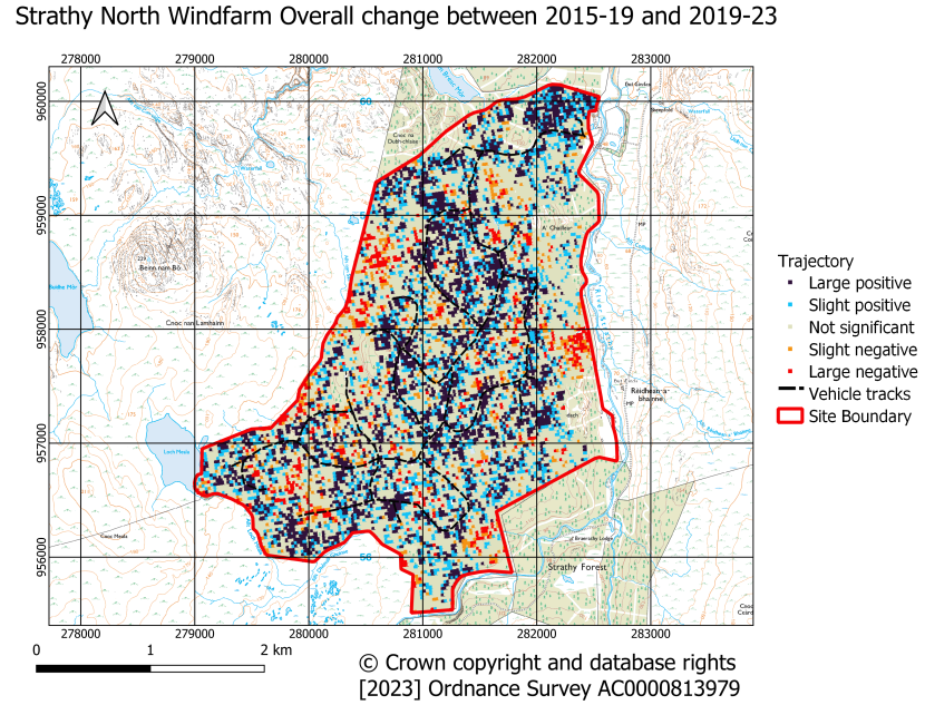
Figure 61: Strathy North Windfarm overall trajectory of change map based on comparison of the periods 2015-19 and 2019-23.
Click for a full description
Strathy North Windfarm overall trajectory of change map based on comparison of the periods 2015-19 and 2019-23. Areas of positive change are widespread and often closely associated with access roads.
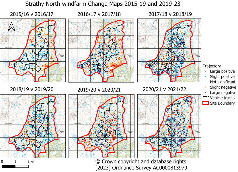
Figure 62: Strathy North Windfarm sequential annual trajectories of change from 2015 to 2023.
Click for a full description
Strathy North Windfarm sequential annual trajectories of change from 2015 to 2023. Areas of positive change are notably associated with access roads in 2017-18 and become more widespread in 2018-19. Negative change occurs in more discrete patches notably along the southeastern edge in 2017-18 and the eastern edge in 2021-22.
| Bog type | Landcover | Periods of restoration and methods used | Condition (Fig. 59 and 60) | Overall trajectory of change (Fig. 61) | Sequential change (Fig. 62) |
|---|---|---|---|---|---|
| Blanket bog | Felled forestry, semi-natural, windfarm infrastructure | No data provided | 2015-19 Compartmentalised, mixed mainly degrading and stiff. Stiff occurs typically on steeper slopes and along roads. 2019-23 Compartmentalised. In comparison to previous period area degrading has reduced, area in good condition has expanded and stiff peat has become more localised to roads, giving a sharper definition to the road network. Contrasting condition is observed across some roads (Figure 59 locations A, B, C) with better condition developing on the upslope side and degrading condition being sustained on the downslope side of the stiff road. | Positive change associated with the road network | No distinct spatial pattern but typically more positive change is associated with the area containing infrastructure in the centre of the site. |
Interpretation
This is a complex site with infrastructure development appearing to have compartmentalised the peatland hydrology.
Roads appear to have consolidated over time, in places creating an effective hydrological barrier that results in water being retained upslope from the road and water being lost downslope from the road, leading to better conditions developing upslope and degrading being maintained downslope. The net result of this appears to be more water retention and expansion of good condition across the site. It may also have resulted in expansion of the area of peat in good condition associated with the small pool system in the southwest of the site (Figure 59 location C). Analysis of the effects of vehicles tracks requires detailed consideration of the topography. The examples given occur where the track runs approximately parallel to the topographic contours, but other more complex examples can be found.
Association of positive change with the road network may be the result of consolidation of the roads post construction. Other areas of stiff peat are clearly associated with steeper slopes along the eastern edge of the site.
Flow Country World Heritage Site
This area covers c.187,000 ha (Figure 63); observations and interpretation are presented for the whole area. Detailed analysis of the many smaller-scale features, restoration projects and local changes in land management are beyond the scope of the project.
Location
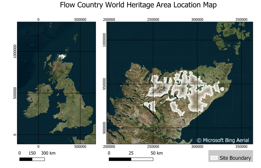
Figure 63: Flow Country World Heritage Site map showing site boundary.
Click for a full description
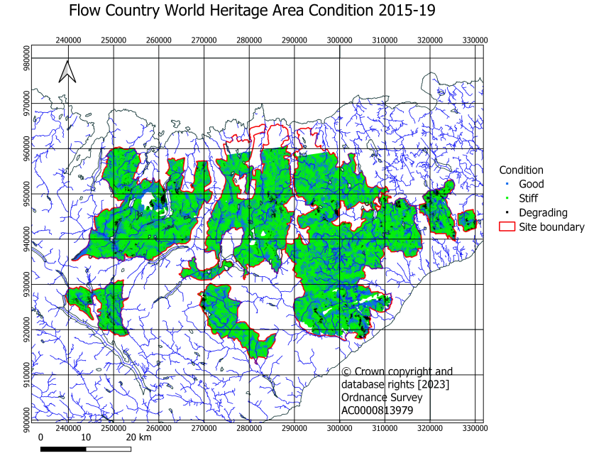
Figure 64: Flow Country World Heritage Site maximum probability condition map for the period 2015-19.
Click for a full description
Flow Country World Heritage Site maximum probability condition map for the period 2015-19. Stiff conditions are widespread, degrading conditions are highly localised and occur mainly in areas of former forestry and good conditions are widely scattered. In detail, the good conditions are often associated with pool systems and in the western part of the area are found on valley floors. Stiffer conditions are typically associated with steeper ground and degraded upland peat.
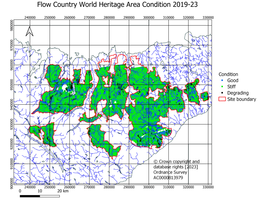
Figure 65: Flow Country World Heritage Site maximum probability condition map for the period 2019-23.
Click for a full description
Flow Country World Heritage Site. Stiff conditions are widespread, degrading conditions are highly localised and occur mainly in areas of former forestry and good conditions are widely scattered. In detail, the good conditions are often associated with pool systems and in the western part of the area are found on valley floors. Stiffer conditions are typically associated with steeper ground and degraded upland peat.
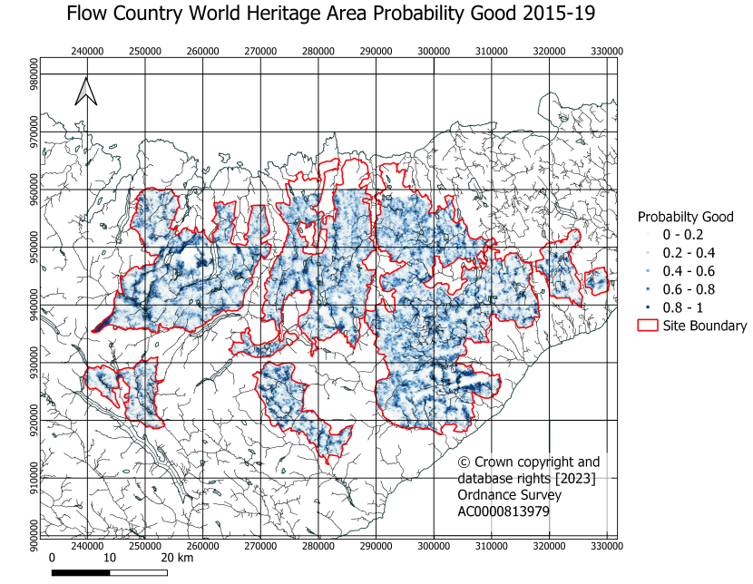
Figure 66: Flow Country World Heritage Site probability condition map for the period 2015-19. Probabilities are shown for the good class.
Click for a full description
Flow Country World Heritage Site probability condition map for the period 2015-19. Probabilities are shown for the good class. Moderate to high probabilities of good condition are widespread. Areas with a moderate to high probability of being in good condition tend to follow trends in the landscape particularly valleys and trends determined by the underlying geological structure of the area.
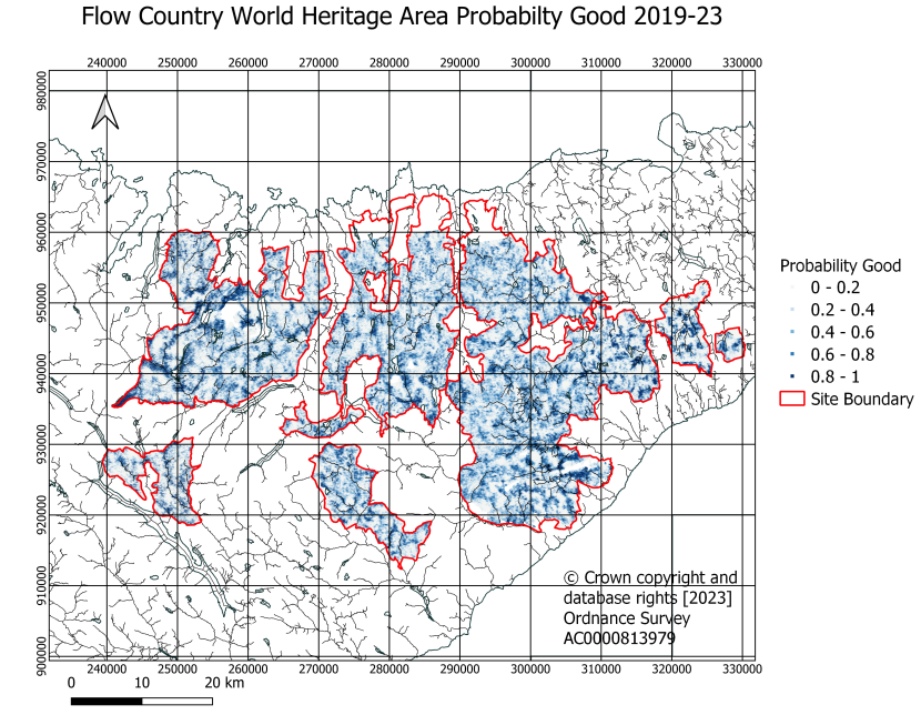
Figure 67: Flow Country World Heritage Site probability condition map for the period 2019-23. Probabilities are shown for the good class.
Click for a full description
Flow Country World Heritage Site probability condition map for the period 2019-23. Probabilities are shown for the good class. Moderate to high probabilities of good condition are widespread. Areas with a moderate to high probability of being in good condition tend to follow trends in the landscape particularly valleys and similar trends determined by the underlying geological structure of the area.

Figure 68: Flow Country World Heritage Site probability condition map for the period 2015-19. Probabilities are shown for the stiff class.
Click for a full description
Flow Country World Heritage Site probability condition map for the periods 2015-19. Probabilities are shown for the stiff class. Moderate to high probabilities of stiff condition are widespread. Areas with a moderate to high probability are typically found on steeper ground, higher hilltops, and in areas of eroded peat.
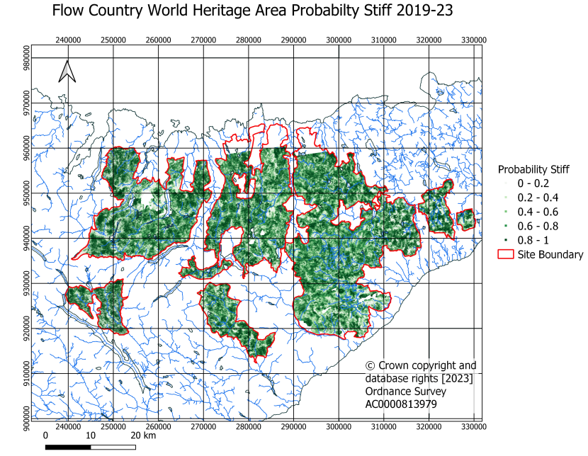
Figure 69: Flow Country World Heritage Site probability condition map for the period 2019-23. Probabilities are shown for the stiff class.
Click for a full description
Flow Country World Heritage Site. Probabilities are shown for the stiff class. Moderate to high probabilities of stiff condition are widespread. Areas with a moderate to high probability are typically found on steeper ground, higher hilltops, and in areas of eroded peat.
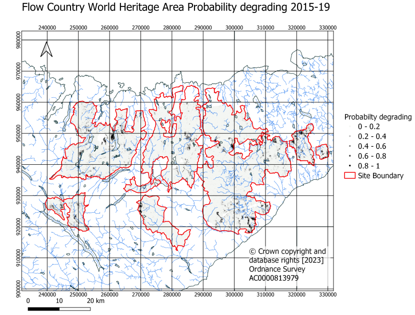
Figure 70: Flow Country World Heritage Site probability condition map for the period 2015-19. Probabilities are shown for the degrading class.
Click for a full description
Flow Country World Heritage Site probability condition map for the period 2015-19. Probabilities are shown for the degrading class. Areas of degrading peat are typically associated with areas of felled forestry, upstream extension of drainage lines close to their source regions and areas of possible mass movement.
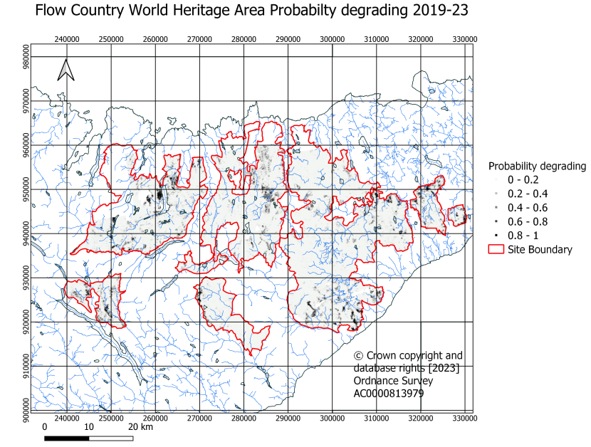
Figure 71: Flow Country World Heritage Site probability condition map for the period 2019-23. Probabilities are shown for the degrading class.
Click for a full description
Flow Country World Heritage Site probability condition map for the period 2019-23. Probabilities are shown for the degrading class. Areas of degrading peat are typically associated with areas of felled forestry, upstream extension of drainage lines close to their source regions and areas of possible mass movement.
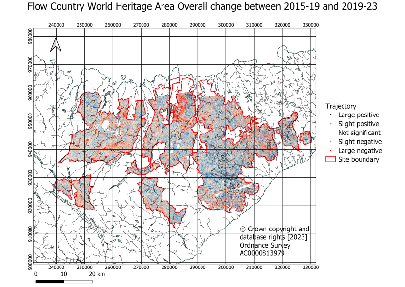
Figure 72: Flow Country World Heritage Site overall trajectory of change map based on comparison of the periods 2015-19 and 2019-23.
Click for a full description
Country World Heritage Site overall trajectory of change map based on comparison of the periods 2015-19 and 2019-23. A distinct patch of negative change in the centre north of the area corresponds to the area of an extensive fire in 2019. Other areas of notable negative change are associated with drainage lines and areas of felled forestry. Discrete areas of positive change associated with restoration work are present but are hard to see on this scale of observation.

Figure 73: Flow Country World Heritage Site annual trajectory of change based on comparison of 2015-16 with 2016-17.
Click for a full description
Flow Country World Heritage Site trajectory of change based on comparison of 2015-16 with 2016-17. Change on this map is very muted, a common observation for change trajectory data observed in this period and we believe this may be due to issues associated with data collected during the first year of satellite operation.
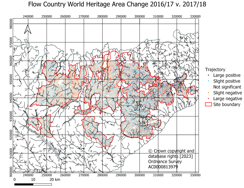
Figure 74: Flow Country World Heritage Site annual trajectory of change based on comparison of 2016-17 with 2017-18.
Click for a full description
Flow Country World Heritage Site annual trajectory of change based on comparison of 2016-17 with 2017-18. Small areas of large negative change correspond to pool systems where the peat subsided substantially on account of the 2018 drought.

Figure 75: Flow Country World Heritage Site annual trajectory of change based on comparison of 2017-18 with 2018-19.
Click for a full description
Flow Country World Heritage Site annual trajectory of change based on comparison of 2017-18 with 2018-19. Extensive positive change represents a rebound of the surface in 2019 following the 2018 drought.
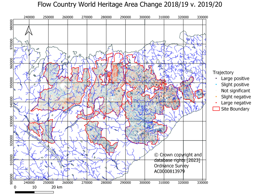
Figure 76: Flow Country World Heritage Site annual trajectory of change based on comparison of 2018-19 with 2019-20.
Click for a full description
Flow Country World Heritage Site annual trajectory of change based on comparison of 2018-19 with 2019-20. A large area of negative change in the centre north of the area corresponds to the area of fire damage in 2019.

Figure 77: Flow Country World Heritage Site annual trajectory of change based on comparison of 2019-20 with 2020-21.
Click for a full description
Flow Country World Heritage Site annual trajectory of change based on comparison of 2019-20 with 2020-21. Small areas of large negative change correspond to pool systems where the peat subsided substantially on account of a very dry spring in 2021.

Figure 78: Flow Country World Heritage Site annual trajectory of change based on comparison of 2020-21 with 2021-22.
Click for a full description
Flow Country World Heritage Site annual trajectory of change based on comparison of 2020-21 with 2021-22. No distinct patterns of behaviour are noted at the scale of observation.
Click here for a larger version of Figure 78.
Observations
The following features are noted and interpreted as follows:
Maximum probability maps (Figures 64 and 65)
- Peat in degrading condition is associated with well-defined areas. On closer inspection these are associated with forestry, forestry removal or distinct (historical) drainage. Some areas may also be associated with mass movement (landslide) particularly in the vicinity of Morven and the upper Langwell Water.
- Peat in good condition is widely dispersed in the eastern and southern parts of the site, and more confined to valleys in the west.
- Peat in stiff condition is dominant.
- As expected, almost all pool systems are classified as containing peat in good condition.
- In eastern areas linear trends in the distribution of peat in good condition correspond to linear trends in the underlying geology that are also represented in the distribution of pool systems. This demonstrates an underlying structural and landscape control on peatland hydrology. This is best observed at slightly higher resolution using a GIS interface.
- At the scale of the maps, overall pattern of peat condition remains similar. Detailed changes associated with local land management are only visible at higher resolution.
Condition probability maps
- Areas with the greatest probability of being in good condition (Figures 66 and 67) frequently occur over pool systems and over valley floors in the western part of the site where the mountains are generally higher and steeper promoting rapid runoff and flow towards the valley floors.
- Areas with the highest probability of being in stiff condition (Figures 68 and 69) frequently occur on margins, steep slopes, hill tops and within areas of eroded peat.
- Areas with the highest probability of being in degrading (Figures 70 and 71) condition correspond to areas of drainage, felled forestry and the upper extension of natural drainage lines. Some areas also appear to correspond to areas of mass movement where subsidence is picking up the vertical component of this motion.
- The largest change between periods of observation is the increasing probability of eroded peat on the upslope extension of natural drainage lines.
Overall change (Figure 72)
- There appears to be generally more negative change at the periphery of the area and along natural margins.
- An extensive area of large negative change in the northern central part of the site corresponds precisely to the area of a large wildfire that occurred in May 2019.
- Other areas with extensive and localised large negative change are associated with drainage or clear-felling.
- There are no areas of extensive large positive change clearly defined on the scale of the map (Figure 72) however at higher resolution many of the areas of peatland restoration within the Forsinard RSPB reserve display large positive change.
Sequential change
- Very little change is observed in 2016/17 when compared to 2015/16 (Figure 73) and this is a general observation across all maps showing change in this period. We therefore propose that this may be due to lower quality satellite data in 2015/16 during which period gaps in collection were more frequent and consequently the time series less well defined.
- The key feature of the sequential change maps are localised areas of either intense negative change in 2017/18 (Figure 74) and 2020/21 (Figure 77) and positive change 2018/19 (Figure 75) and 2019/20 (Figure 76). Many of these areas are identical and correspond to pool systems or areas of long-term restoration. The reason for this is capacity of the areas considered to be in the best condition to adapt to weather events, notably the spring drought of 2018 and the summer drought of 2021. As observed in the field (Marshall et al., 2022), periods of drought cause marked subsidence of the pool systems resulting in irreversible compaction and intense and extensive rewetting in the following winters.
- The area of the Flow Country fire in the central northern part of the site also displays prominent negative change in the year of the fire 2018/19 (Figure 75) and subsequent year 2019/20 (Figure 76).
- Little in the way of distinct patterns of change are observed in 2021/22 (Figure 78) which was a second dry summer in succession. This may indicate that the system had a reduced capacity for further adaptation.
Discussion and evaluation
The methods provide an objective, repeatable and data-driven approach to the classification of peatland condition and trajectories of change. Objectivity and repeatability are advantageous compared to field observations which, although of immense value, are prone to subjectivity on account of many factors including unconscious bias, level of expertise, and weather conditions encountered on the day. The same area may therefore be classified differently by two independent observers, adding uncertainty and reducing the repeatability of field-based assessments compared with the InSAR approach.
The methods also provide a useful view of peatland grounded in the resilience mechanism that arises from the coupling mechanical-ecological-hydrological behaviours. This is somewhat different from the traditional views grounded in ecology and/or hydrology (e.g. NVC categories) or defined by land management and intervention (e.g. Peatland Code). For example, the classification of good condition implies a high amplitude swelling of the surface in response to water storage in winter, with no sustained long-term subsidence. Although this is typical of Sphagnum dominated peatland in the best condition, the presence of Sphagnum is not implicit in the classification, which could equally indicate any spongy wet area. The IPCC and Peatland Code use broad land-use classifications like eroding, drained, modified and near-natural that understandably have a practical use. However, such classifications say little about the ecological-hydrological-mechanical properties of the peat which can vary considerably within each class and determine inherent resilience to drought or fire. The nuances that the InSAR approach can pick out may be useful to further develop our understanding of, for example, area of influence of drains, restoration intervention, tracks, etc. The InSAR approach also provides a potential framework for the identification of areas with high restoration potential as well as likely target conditions, based on the natural tendency of the system to hold water.
The classification schemes were purposefully chosen to be simple and meaningful, with gradational change illustrated via robust estimates of probability or measures of change. More complex classification schemes could have been derived from the same data. To those who prefer detailed ecological subdivision this may seem inadequate, but in our opinion the ecological data augments the “bog breathing” classification and vice versa, both providing equally useful information on the state of the peat. Bog breathing is the only method that represents the physical poroelastic state of the peat which is crucial to resilient behaviour.
The coupling of mechanics, ecology and hydrology requires and forces the person interpreting the data to think more broadly about these interactions and to consider contextual data. For example, an uneven response to restoration will probably be related to the topography and hydrology of a site with lower and flatter areas at the base of a slope rewetting more readily. In terms of change, failure of a restoration site to show rapid positive change or vice versa needs to be considered in the context of the time since restoration, intensity of restoration, topography, and post-restoration weather conditions and land management.
Ultimately the success of any remote sensing method should be measured in terms of usefulness, rather than on the level of detail it provides. We therefore evaluate usefulness with respect to the following applications.
Usefulness of maps for identifying priority restoration areas
Given limited budgets a useful classification could help the user identify areas that will give a maximum return on the investment in restoration. Success in this context can be defined in many ways but for the purpose of evaluating this method the following is appropriate:
- Enable identification of areas that will respond well to restoration.
- To achieve this the method differentiates areas that are in variable condition within areas that are given broad brush classifications. For example, eroding, gullied areas of peat hags are viewed as general priority for peatland restoration and potential carbon credits. These areas can be classed as degrading, but more often are classed as being in stiff or good condition which superficially clashes with the general idea that these areas would be prioritised for restoration. These areas are particularly interesting as there is uncertainty as to the relative influence of land management vs. natural processes in determining the condition of the peat. It is for this reason that the classification is useful as it differentiates condition within the eroded landscape. For example:
- Eroded peat classed as stiff can reasonably be presumed to have reached a high level of prolonged degradation, compaction and relative stability with the dominant forces of degradation being erosion by water and wind rather than drainage and oxidation. Full depth rewetting of this peat could be potentially hazardous, and the focus of restoration should arguably be more on stabilisation and re-establishment of peat accumulation in the base of gullies.
- Areas of eroded peat classed as good, are most likely to be experiencing or be prone to natural recovery between hags in which case it may be better reducing pressures that accentuate erosion (e.g. grazing) and recognising that a natural regeneration is underway.
- Areas of eroded peat that are classed as actively degrading are probably most in need of urgent restoration and therefore higher priority.
- As the classes are based on the behaviour of the surface in response to hydrology and not vegetation community, the result can be used to identify areas with favourable hydrology most likely to respond to ecological restoration on account of their natural tendency to hold water. For example.
- Within areas of established forestry, it is not unusual to observe patches of land in good condition (e.g. areas that were too wet to be drained initially). This tallies with personal observations of variation in the wetness of the understorey and rides. On felling, these areas are likely to respond most favourably to restoration.
- Some drained areas appear in good condition, most likely on account of poor maintenance of drains in areas that naturally re-wet. These areas may require less intervention or potentially could be left to recover with minimal or no intervention. Field checking may be advisable.
- Old areas of (hand) peat cutting where peat may be starting to naturally re-establish. Again, these areas may require minimal intervention.
- Areas that are actively degrading are clearly identified and should be a priority. In these areas, degradation is mostly the occurring response to known land management activities. The evidence provided is therefore useful in communicating the need for restoration to land managers.
- To achieve this the method differentiates areas that are in variable condition within areas that are given broad brush classifications. For example, eroding, gullied areas of peat hags are viewed as general priority for peatland restoration and potential carbon credits. These areas can be classed as degrading, but more often are classed as being in stiff or good condition which superficially clashes with the general idea that these areas would be prioritised for restoration. These areas are particularly interesting as there is uncertainty as to the relative influence of land management vs. natural processes in determining the condition of the peat. It is for this reason that the classification is useful as it differentiates condition within the eroded landscape. For example:
Usefulness of the change detection method for tracking recovery
Change detection works well, displaying expected positive and negative changes to restoration, fire and weather. It therefore provides easily communicated evidence as to the effectiveness of restoration work and different restoration techniques (Mitchell et al., 2025). Of note, it can display positive change even in areas where restoration progress is likely to be slow and the result is more likely to be stabilisation of eroding stiff peat than establishment of spongy, wet, good conditions.
Contextual information is crucial if change is to be understood. Change detection is able to provide this contextual information from the surrounding landscape and concurrent weather. For example, a lack of response to restoration may be explained by drought conditions causing negative change in the wider near natural elements of the peat landscape.
Change detection provides a means of evaluating the short-term effectiveness of restoration strategies. For example, Mitchell et al. (2025) showed, using change detection data from the Whitelee Windfarm, that wave-damming techniques were less prone to negative change than standard drain blocking techniques when subject to the same weather conditions.
Change detection provides insight into the process of restoration. Following restoration, the initial consequence of restoration can appear quite negative, and the speed of response appears to be strongly influenced by position within the landscape. Both at Tardoes Farm and Strathy, restoration on steeper slopes appears to have generated InSAR outputs showing negative change and poor condition, which may be temporary, but nonetheless indicates that the response varies according to topography. Similarly, areas showing rapid positive change tend to be flatter areas where water naturally accumulates.
A notable aspect of change detection is the different periods over which change can be determined. Different periods can be easily selected with shorter periods being more indicative of change due to land management and longer periods more likely to represent climate change. Annual change seems particularly good at elucidating the response to restoration activities. Overall change (first four years vs last four years) which includes an additional nine months in 2022-23 provides a more robust picture of what is happening on a longer period.
Insights gained from general trends in change and condition after restoration
In combination, change detection and condition observations lend insight to the reasonable expected outcomes of restoration:
- On lowland raised bogs, good condition should be the expectation. Low slope angles mean that water should be retained, and stiff peat should only be acceptable at the margins. Positive change in response to restoration should be rapid. This is observed partly or wholly across the three lowland sites.
- On eroded blanket bog stiff peat displays a much slower response to restoration. Interventions, particularly reprofiling appear to stiffen the peat at least in the short term. The most rapid responses appear to occur in response to drain blocking in areas of lower slope angle. A caveat to this observation is that most of the blanket bog sites were restored somewhat later than the lowland raised bogs.
- Stiff peat may be an appropriate end result of restoration on some blanket bog areas, and this needs to be carefully considered relative to topography and potential for instability.
Conclusions
The project has successfully delivered a data product that quantifies peatland condition and the trajectory of change in that condition over a large area of Scotland. The spatial resolution and extent of coverage allow for the use of the outputs at both the local scale, as shown by the raised bog work, and to generate statistics at the landscape or national level.
The results are data driven, objective, quantitative and grounded in a robust statistical framework and summaries of condition and change are easily extracted from the data products.
The outputs are complementary to traditional assessment of peatland condition, and the additional information provided can aid in restoration project design and restoration prioritisation.
A simple classification system is in principle easily understood and inter-related but in detail requires the person interpreting the data to incorporate contextual knowledge of land management, ecology, weather patterns and other events (e.g. fire, track construction) to understand the results. Maps generated need to be informed by timelines of intervention. It cannot be assumed that a shift to degrading status is necessarily bad as it may be a step preceding recovery, following, for example, restoration action.
In the case studies, most observations appear to correspond to expected or known changes that have occurred on the sites.
The results provide insights into the different expectations as to how lowland raised bogs and upland blanket bogs respond to restoration.
Change detection techniques are particularly useful in rapidly assessing whether interventions are causing a change in peatland behaviour on timeframes far shorter than those over which peatland ecological conditions are expected to change. The scale of data capture also allows for comparison with nearby non-restored areas that should enable untangling of the impacts of restoration work and the influence of weather on the outputs.
Potential next steps
- Investigate the range of ground conditions encountered within each class to improve interpretation and understanding.
- Explore the relationship between annual and seasonal weather patterns and changes in condition/trajectory maps compared with actual changes in hydrological and ecological condition.
- Investigate using the OODA statistical framework to integrate additional datasets (e.g. backscatter SAR and optical data) to provide a more nuanced probabilistic classification of condition and water table depth.
References
Almendinger, J.C., Almendinger, J.E. and Glaser, P.H., 1986. Topographic fluctuations across a spring-fen and raised bog in the Lost River peatland, Northern Minnesota Journal of Ecology, 74, 393–401.
Alshammari, L., Large, D.J., Boyd, D.S., Sowter, A., Anderson, R., Andersen, R. and Marsh, S., 2018. Long-term peatland condition assessment via surface motion monitoring using the ISBAS DInSAR technique over the Flow Country, Scotland Remote Sensing,10(7), 1103.
Alshammari, L., Boyd, D.S., Sowter, A., Marshall, C., Andersen, R., Gilbert, P., Marsh, S. and Large, D.J., 2020. Use of surface motion characteristics determined by InSAR to assess peatland condition Journal of Geophysical Research: Biogeosciences, 125, e2018JG004953.
Andersen, R., Poulin, M., Borcard, D., Laiho, R., Laine, J., Vasander, H. and Tuittila, E.T., 2011. Environmental control and spatial structures in peatland vegetation Journal of Vegetation Science, 22(5), 878-890.
Belyea, L.R. and Baird, A.J., 2006. Beyond “the limits to peat bog growth”: Cross‐scale feedback in peatland development Ecological Monographs, 76(3), 299-322.
Bradley, A.V., Andersen, R., Marshall, C., Sowter, A. and Large, D.J., 2022. Identification of typical ecohydrological behaviours using InSAR allows landscape-scale mapping of peatland condition Earth Surface Dynamics, 10(2), 261-277.
Bradley, A.V., Mitchell, E, Dryden, I., Fallaize, I., Islam, T.I, Large, D.J., Andersen, R. and Marshall, C., 2025. Analysis of an InSAR “bog breathing” based classification of peatland condition relative to field observations in Cairnsmore National Nature Reserve NatureScot Research Report 1308.
Evans, C., Artz, R., Burden, A., Clilverd, H., Freeman, B., Heinemeyer, A., Lindsay, R., Morrison, R., Potts, J., Reed, M. and Williamson, J., 2022. Aligning the Peatland Code with the UK peatland inventory Report to Defra and the IUCN Peatland Programme.
Howie, S.A., and Hebda, R.J., 2018. Bog surface oscillation (mire breathing) a useful measure in raised bog restoration Hydrological Processes, 32, 1518-1530.
Hrysiewicz, A., Holohan, E.P., Donohue, S. and Cushnan, H., 2023. SAR and InSAR data linked to soil moisture changes on a temperate raised peatland subjected to a wildfire Remote Sensing of Environment, 29.
Ingram, H.A.P. 1983. Hydrology. in A.J.P. Gore, ed. 1983. Mires: Swamp, Bog, Fen and Moor, vol. 4A, General Studies. New York, Elsevier Science, pp. 67–158.
Islam, M.T., Bradley, A.V., Sowter, A., Andersen, R., Marshall, C., Long, M., Bourke, M.C., Connolly, J. and Large, D.J., 2022. Potential use of APSIS-InSAR measures of the range of vertical surface motion to improve hazard assessment of peat landslides Mires and Peat, 28, 21, 19pp.
Loisel, J., Gallego-Sala, A., 2022. Ecological resilience of restored peatlands to climate change Communications Earth and Environment, 3, 208.
Large, D.J., Bradley, A.V., Islam, M.D., Mitchell, E., Dryden, I., Fallaize, C., Andersen, R. and Marshall, C., 2025. Use of satellite measures of surface motion to improve the assessment of peat landslide susceptibility NatureScot Research Report 1344.
Lees, K.J., Quaife, T., Artz, R.R.E., Khomik, M. and Clark, J.M., 2018. Potential for using remote sensing to estimate carbon fluxes across northern peatlands - A reviewScience of the Total Environment, 615, 857-874.
Lees, K.J., Artz, R.R.E., Chandler, D., Aspinall, T., Boulton, C.A., Buxton, J., Cowie, N.R. and Lenton, T.M., 2021. Using remote sensing to assess peatland resilience by estimating soil surface moisture and drought recovery Science of the Total Environment, 761.
Mahdiyasa, A.W., Large, D.J., Muljadi, B.P., Icardi, M. and Triantafyllou, S., 2022. MPeat—A fully coupled mechanical-ecohydrological model of peatland development Ecohydrology, 15(1), e2361.
Mahdiyasa, A.W., Large, D.J., Muljadi, B.P. and Matteo, I., 2023. Modelling the influence of mechanical-ecohydrological feedback on the nonlinear dynamics of peatlands Ecological Modelling, 478, 110299.
Marshall, C., Bradley, A.V., Andersen, R. and Large, D.J., 2021. Using peatland surface motion (bog breathing) to monitor Peatland Action sites NatureScot Research Report 1269.
Marshall, C., Sterk, H.P., Gilbert, P.J., Andersen, R., Bradley, A.V., Sowter, A., Marsh, S. and Large, D.J., 2022. Multiscale Variability and the Comparison of Ground and Satellite Radar Based Measures of Peatland Surface Motion for Peatland Monitoring Remote Sensing, 14(2), 336.
Mitchell, E.G., Dryden, I.L., Fallaize, C.J., Andersen, R., Bradley, A.V., Large, D.J. and Sowter, A., 2024. Object oriented data analysis of surface motion time series in peatland landscapes Journal of the Royal Statistical Society, Series C.
Mitchell, E., Fallaize, C., Dryden I., Bradley, A.V., Large, D.J., Andersen, R. and Marshall, C., 2025. A summary of surface motion remote sensing methods for the monitoring of peatlandNatureScot Research Report 1355.
Morton, P.A. and Heinemeyer, A., 2019. Bog breathing: the extent of peat shrinkage and expansion on blanket bogs in relation to water table, heather management and dominant vegetation and its implications for carbon stock assessments Wetlands Ecology and Management, 27(4), 467-482.
NatureScot, 2016. Carbon and Peatland 2016 map
Price, J.S., 2003. Role and character of seasonal peat soil deformation on the hydrology of undisturbed and cutover peatlands Water Resources Research, 39(9).
Räsänen A., Tolvanen, A. and Kareksela, S., 2022. Monitoring peatland water table depth with optical and radar satellite imagery International Journal of Applied Earth Observation and Geoinformation, 112(2),102866.
Sowter, A., Bateson, L., Strange, P., Ambrose, K. and Syafiudin, M.F., 2013. DInSAR estimation of land motion using intermittent coherence with application to the South Derbyshire and Leicestershire coalfields Remote Sensing Letters, 4 (10), 979–987.
Sowter, A., Bin Che Amat, M., Cigna, F., Marsh, S., Athab, A. and Alshammari, L., 2016. Mexico City land subsidence in 2014–2015 with Sentinel-1 IW TOPS: Results using the Intermittent SBAS (ISBAS) techniqueInternational Journal of Applied Earth Observation and Geoinformation, 52, 230-242.
Sowter, A., 2023. Email from Andrew Sowter regarding use of the APSIS InSAR method in afforested areas (Personal communication).
Scottish Government. 2023. National Planning Framework 4
Sterk, H.P., Marshall, C., Cowie, N.R., Clutterbuck, B., McIlvenny, J. and Andersen, R., 2023. Blanket bog CO2 flux driven by plant functional type during summer drought Ecohydrology, 16(2), e2503.
Tampuu, T., Praks, J., Uiboupin, R. and Kull, A., 2020. Long Term Interferometric Temporal Coherence and DInSAR Phase in Northern Peatlands Remote Sensing. 12, 1566.
Toca, L., Morrison, K., Artz, R.R.E., Gimona, A. and Quaife, T., 2022. High resolution C-band SAR backscatter response to peatland water table depth and soil moisture: a laboratory experiment International Journal of Remote Sensing, 43, 5231–5251.
Waddington, J.M., Kellner, E., Strack, M. and Price, J.S., 2010. Differential peat deformation, compressibility, and water storage between peatland microforms: Implications for ecosystem function and development Water Resources Research, 46, W07538.
Last updated:


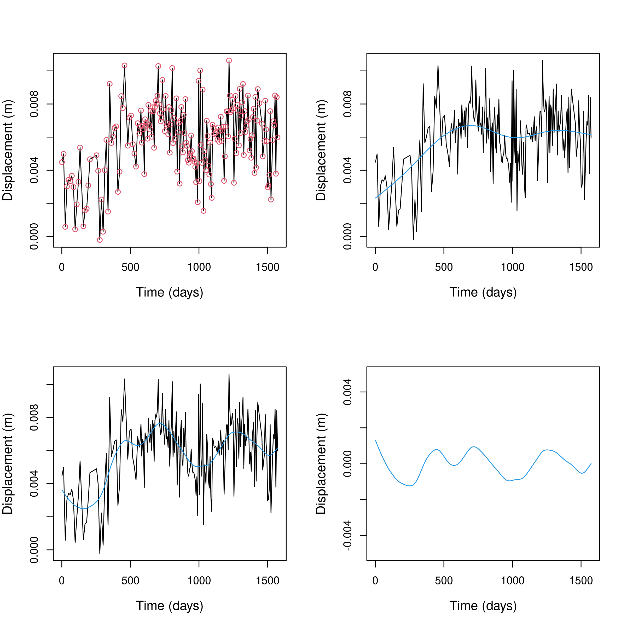
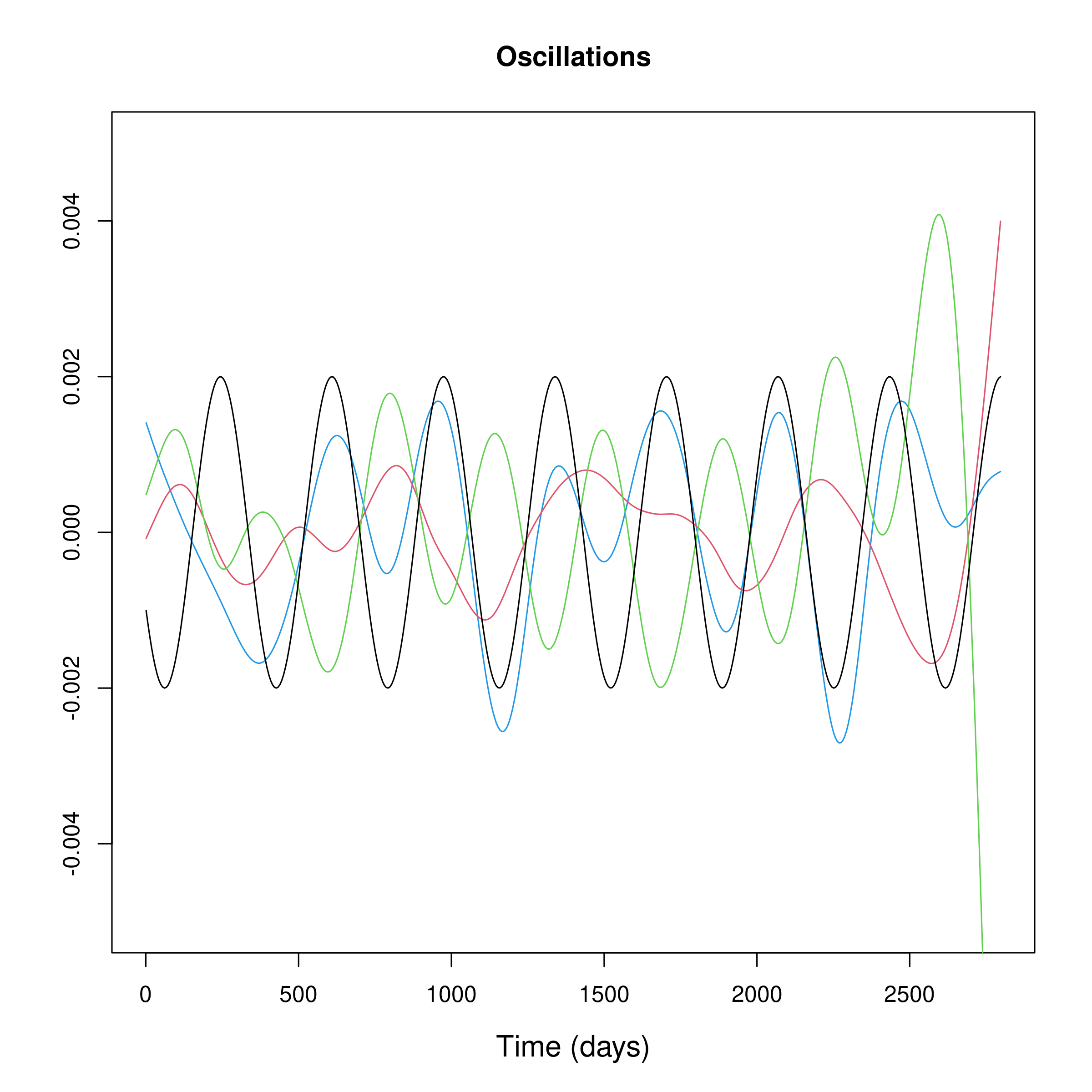
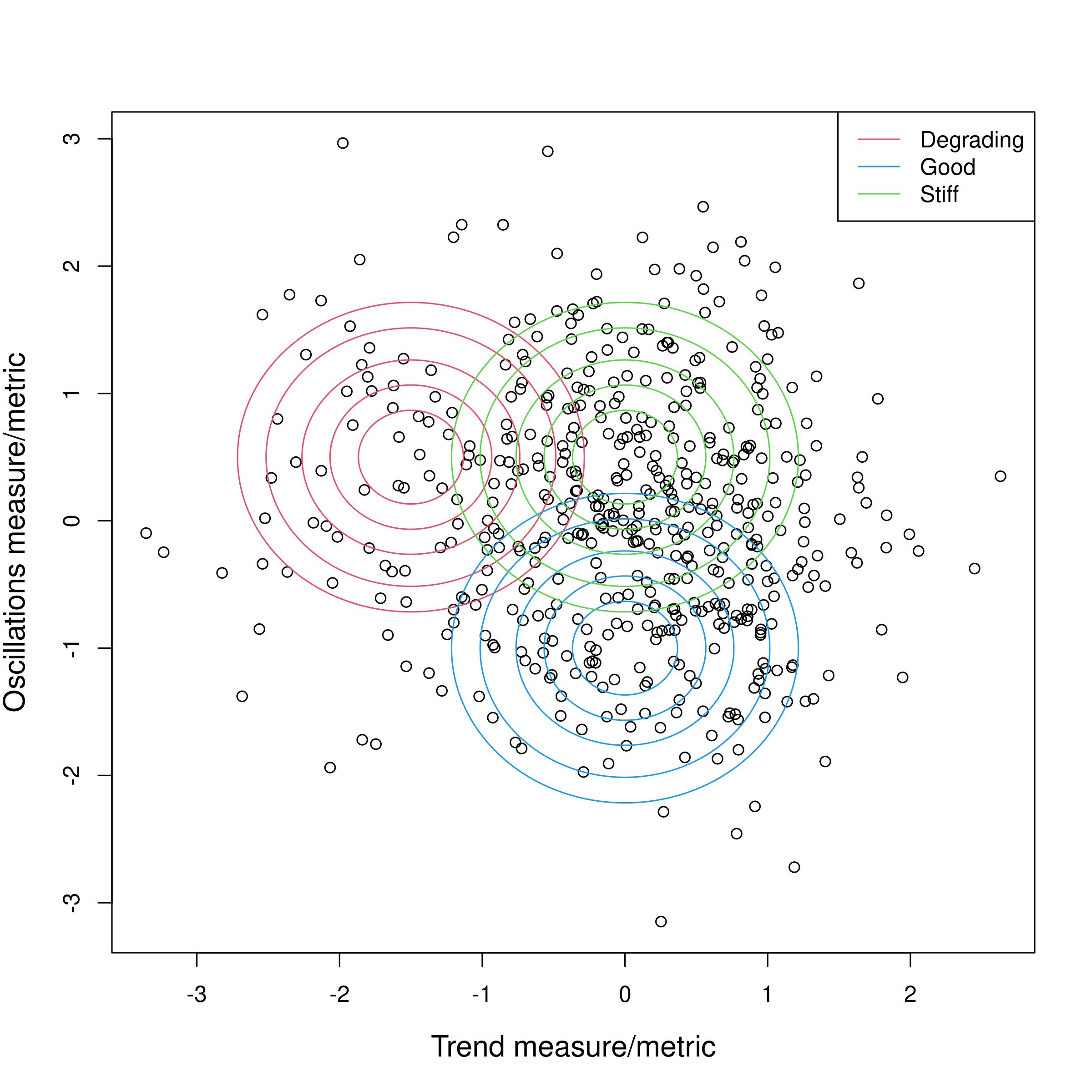
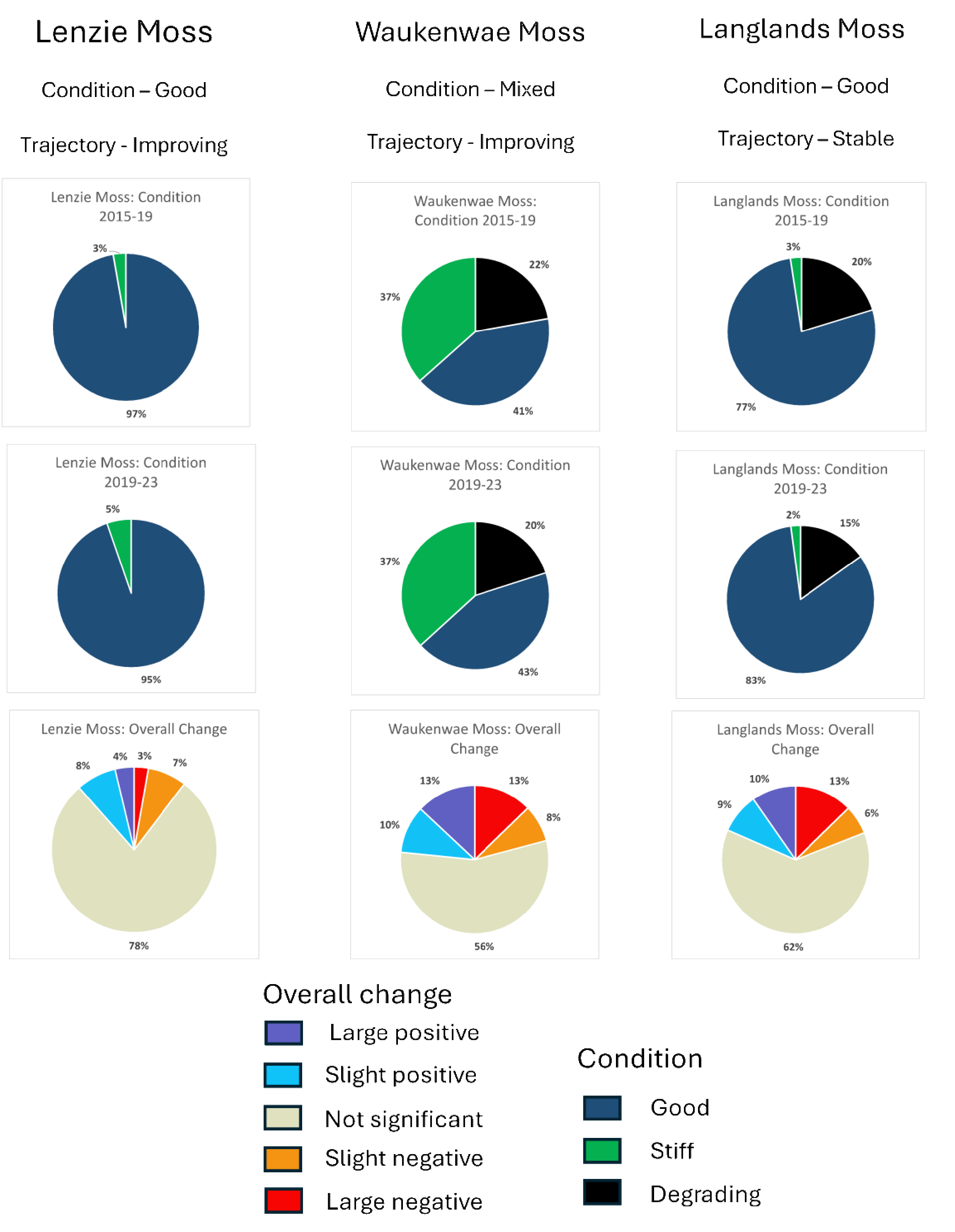
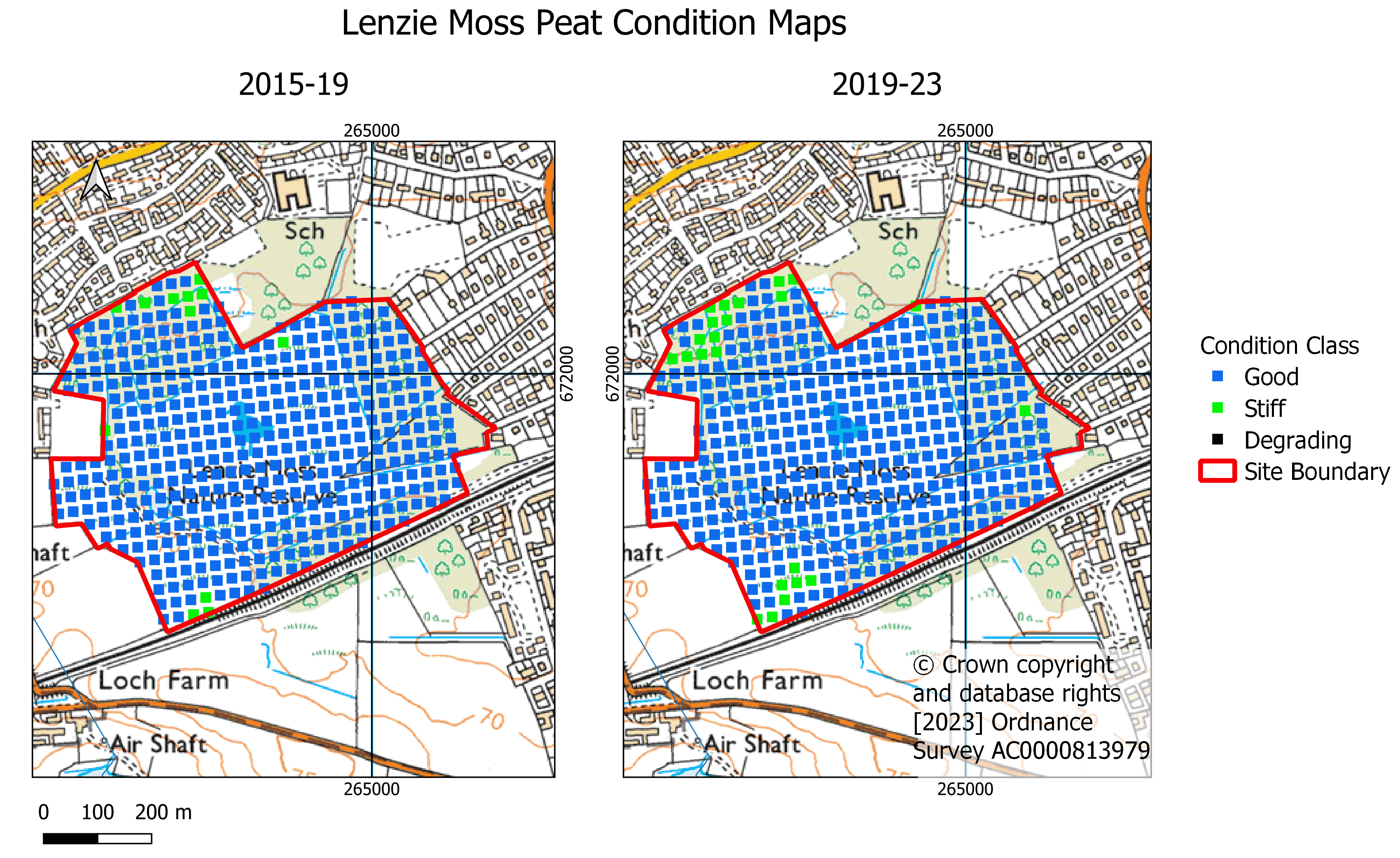
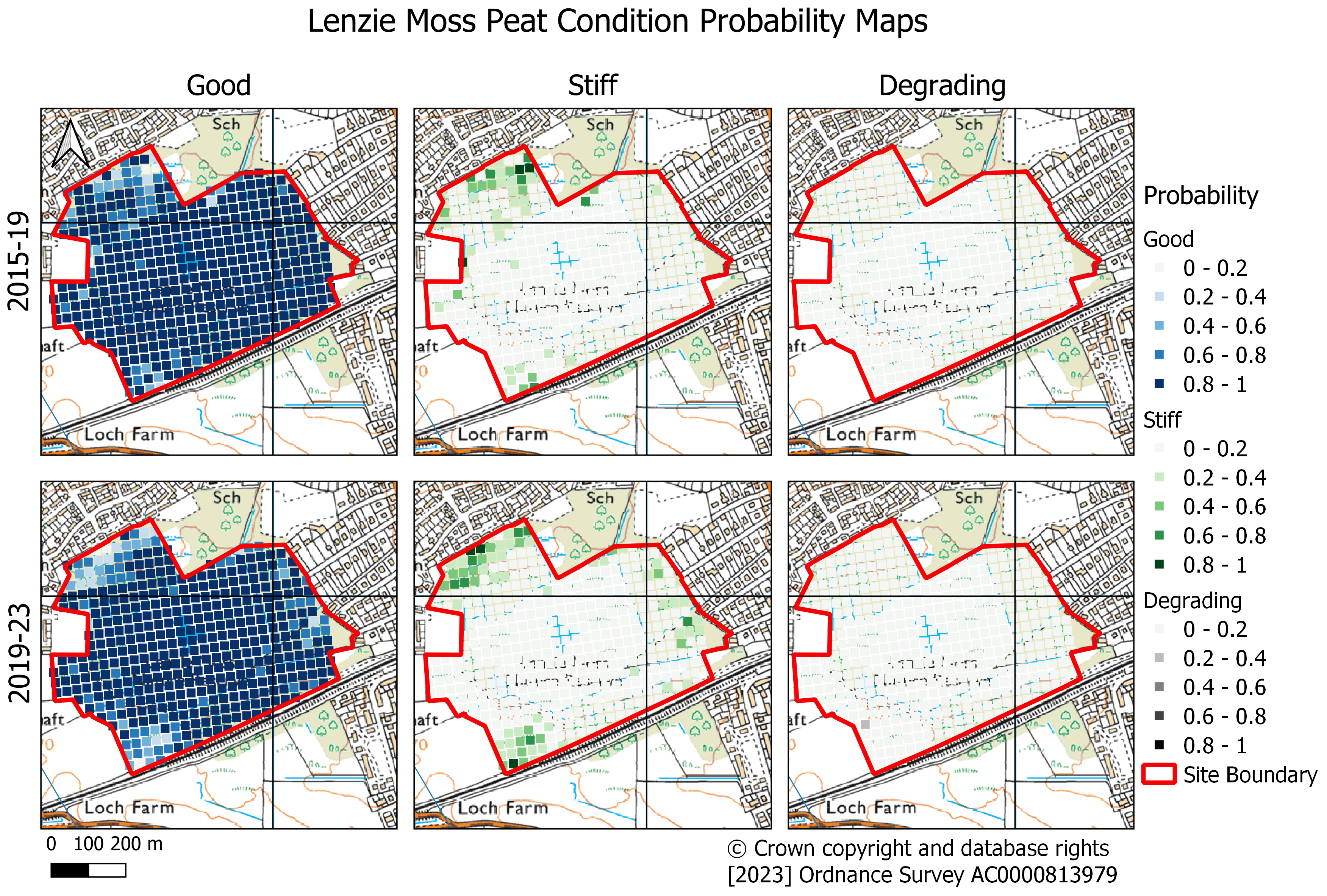
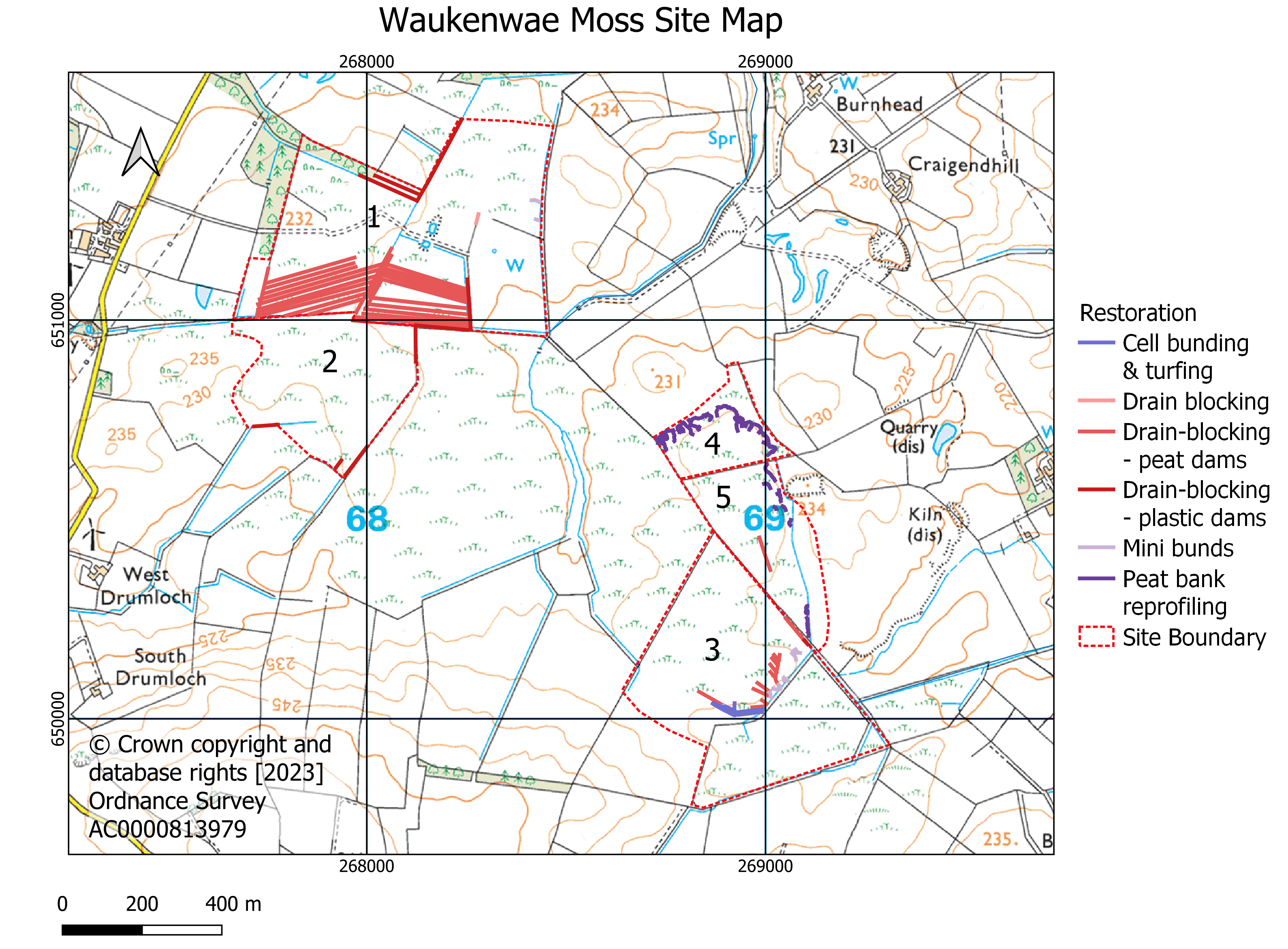
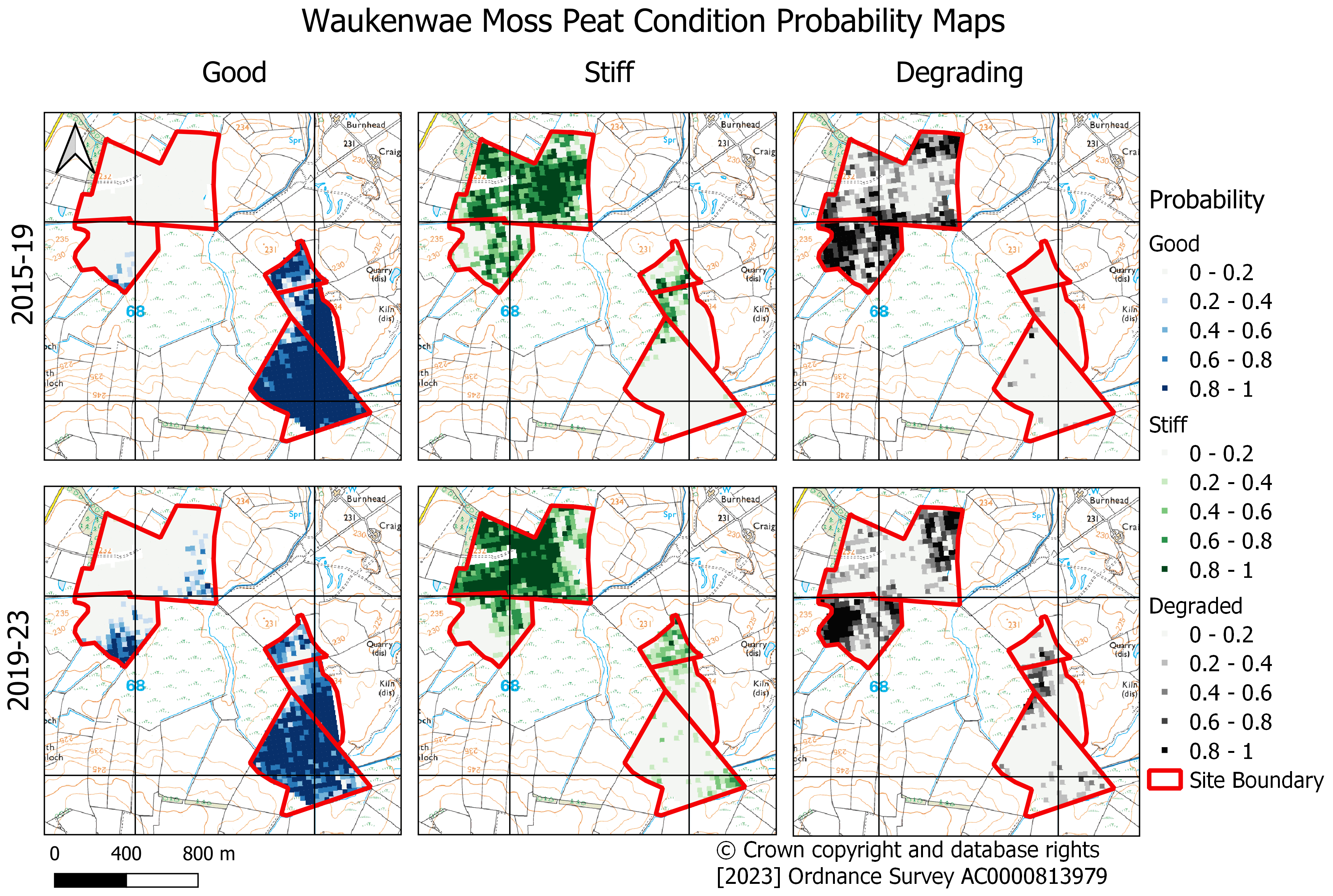
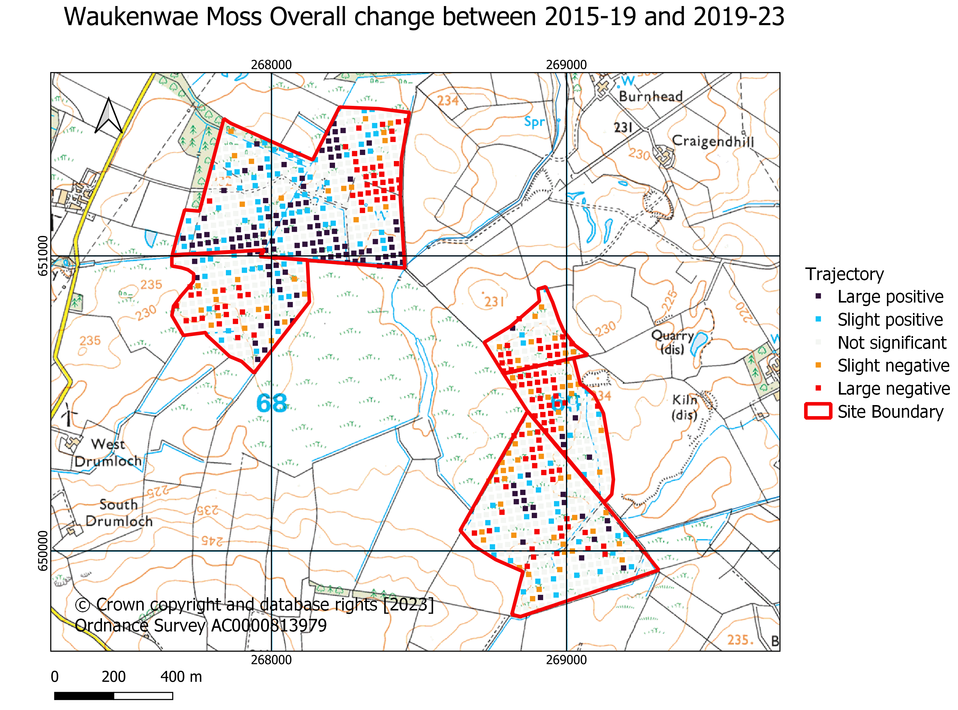
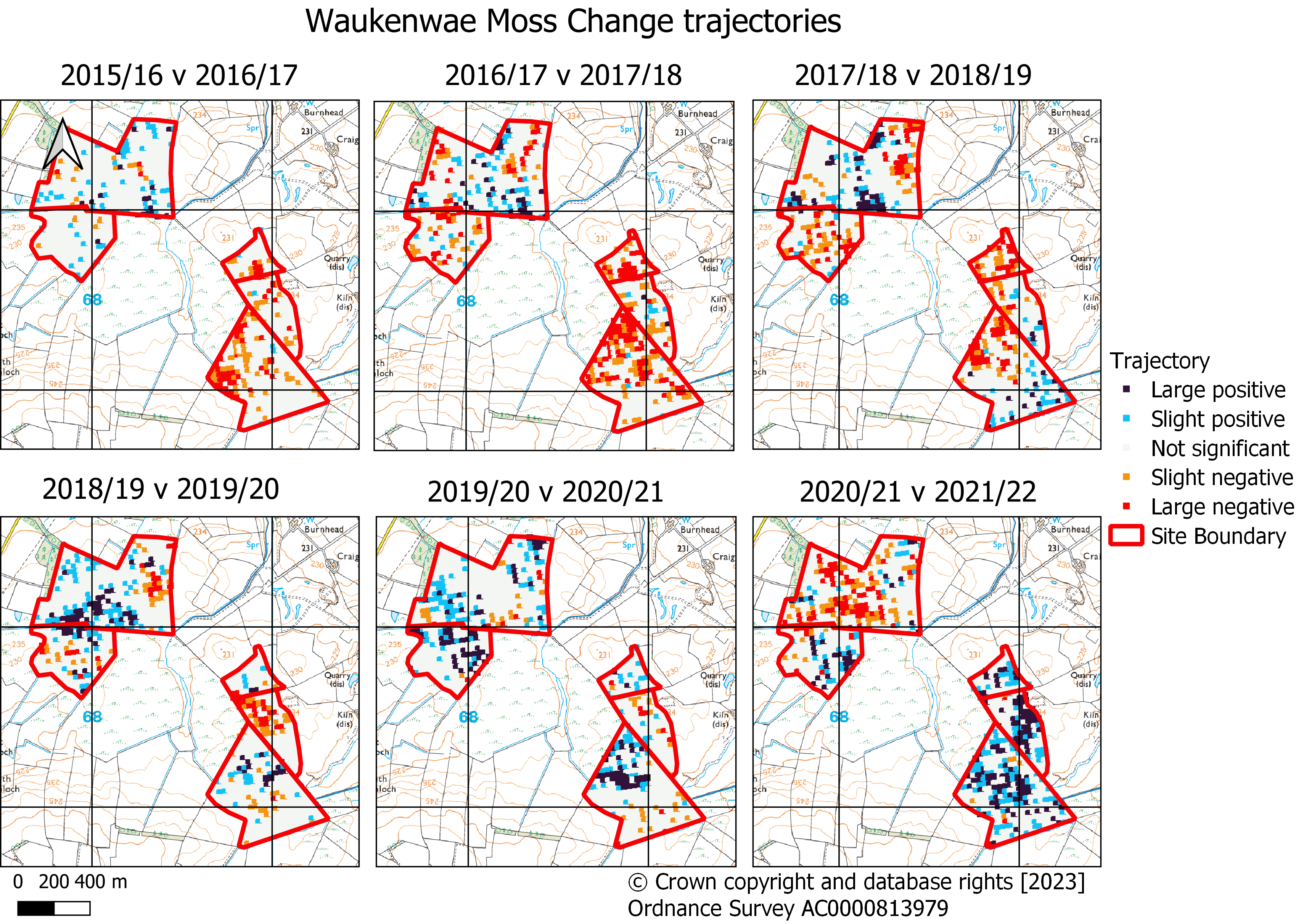
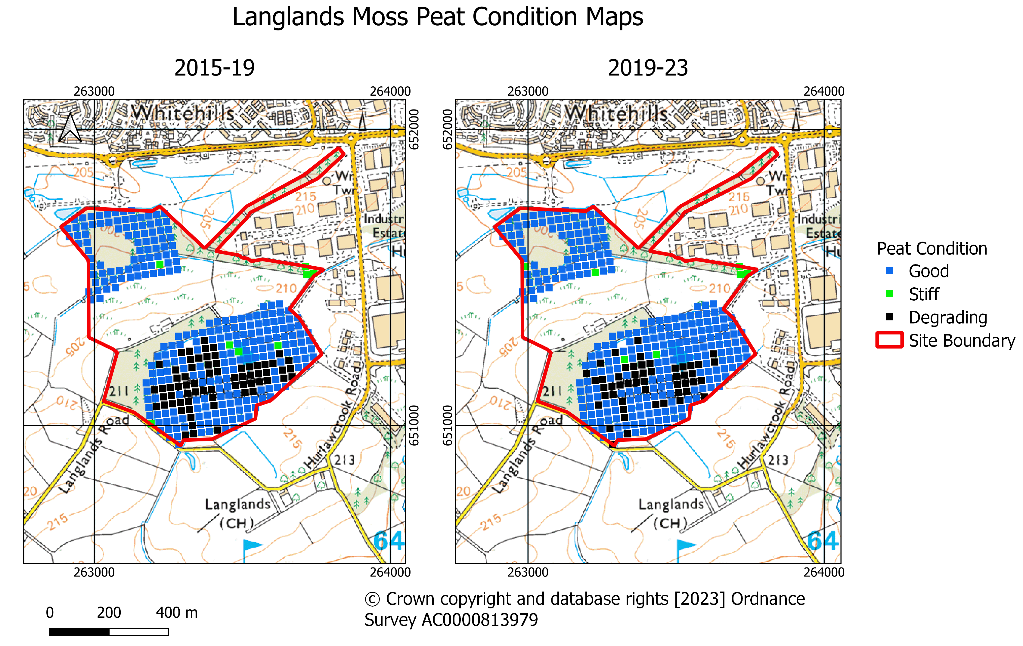
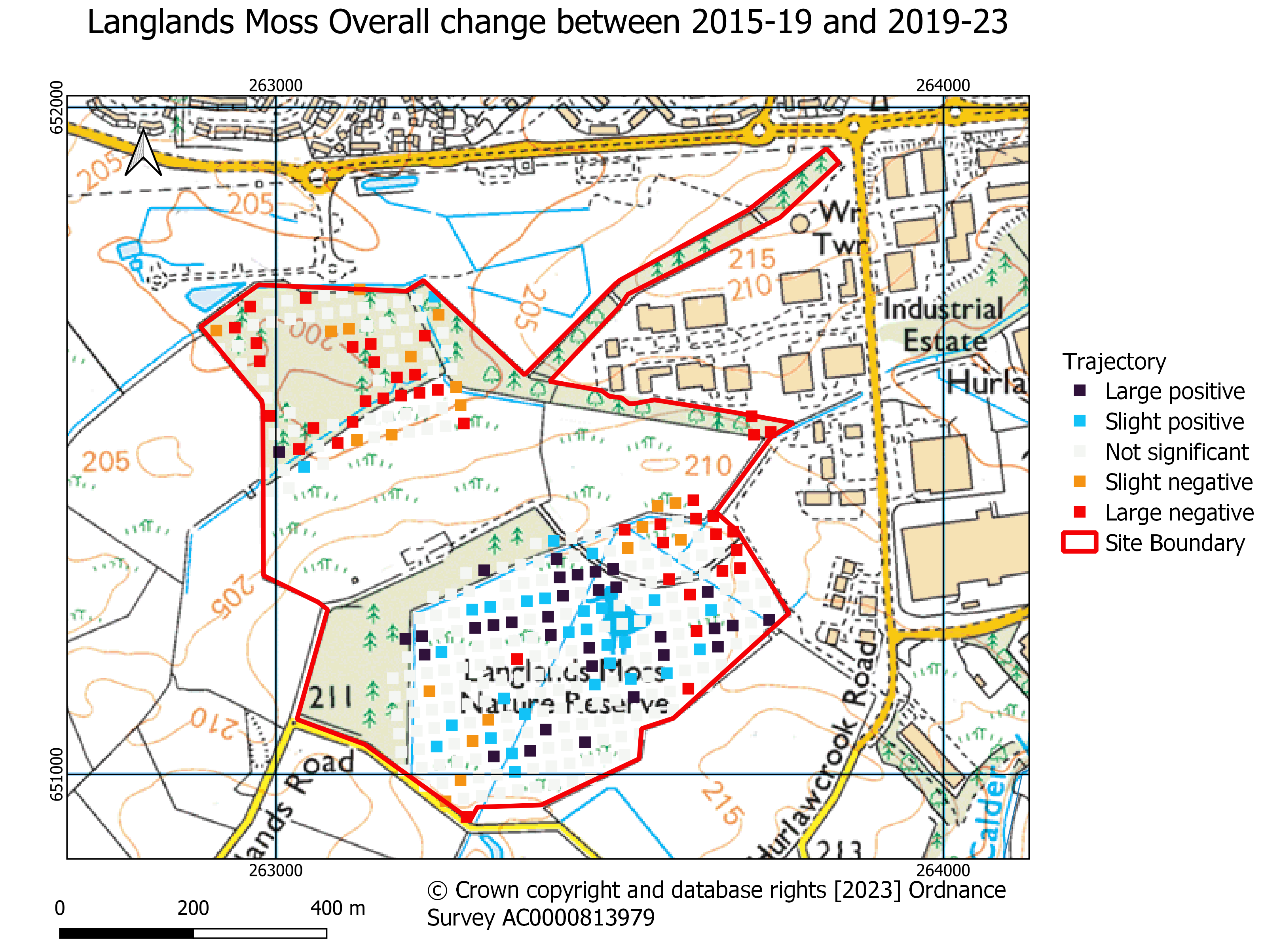
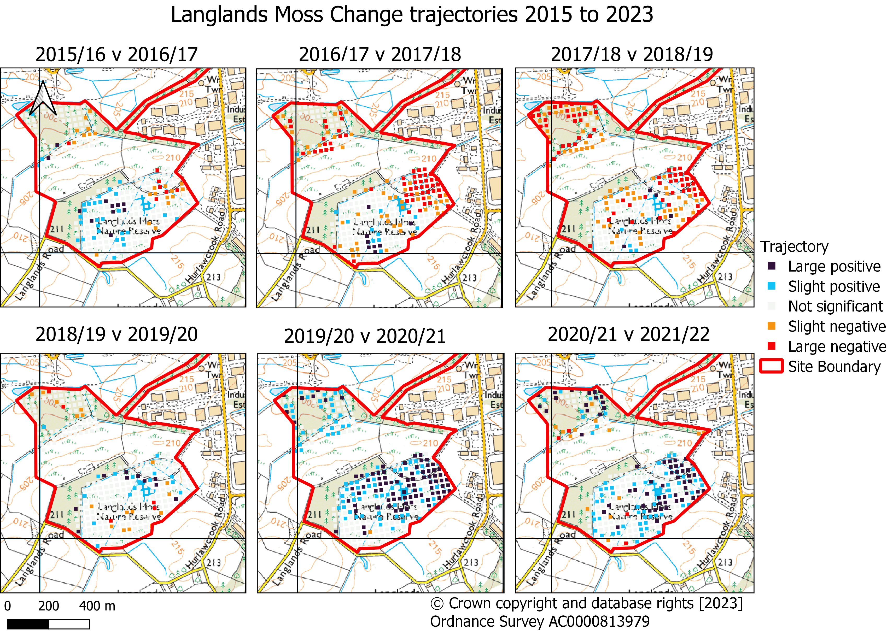
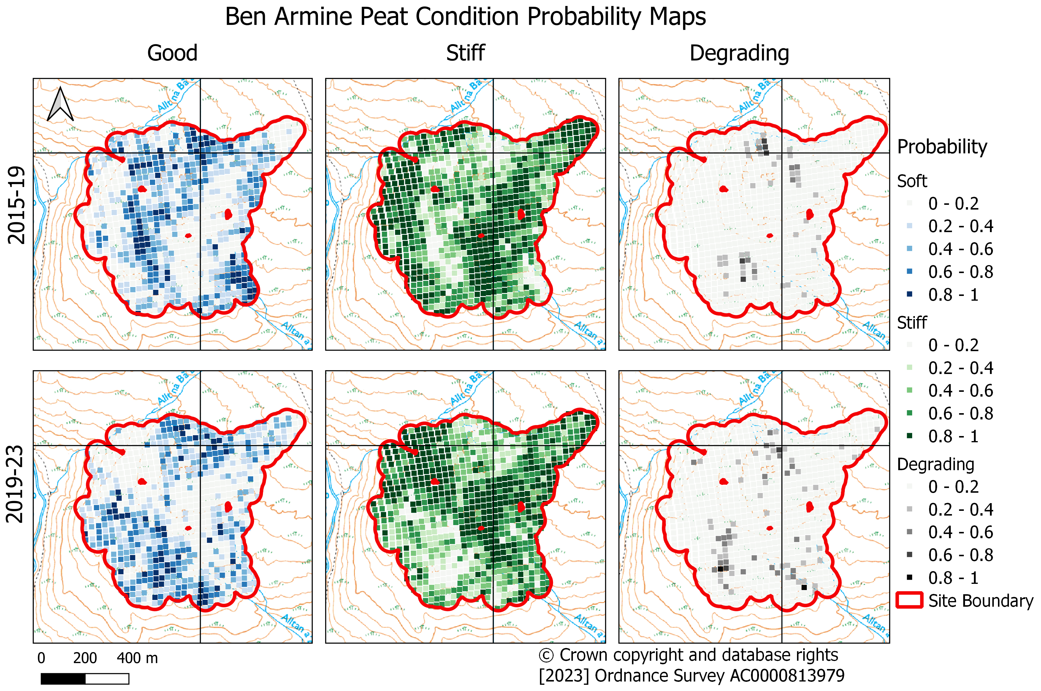
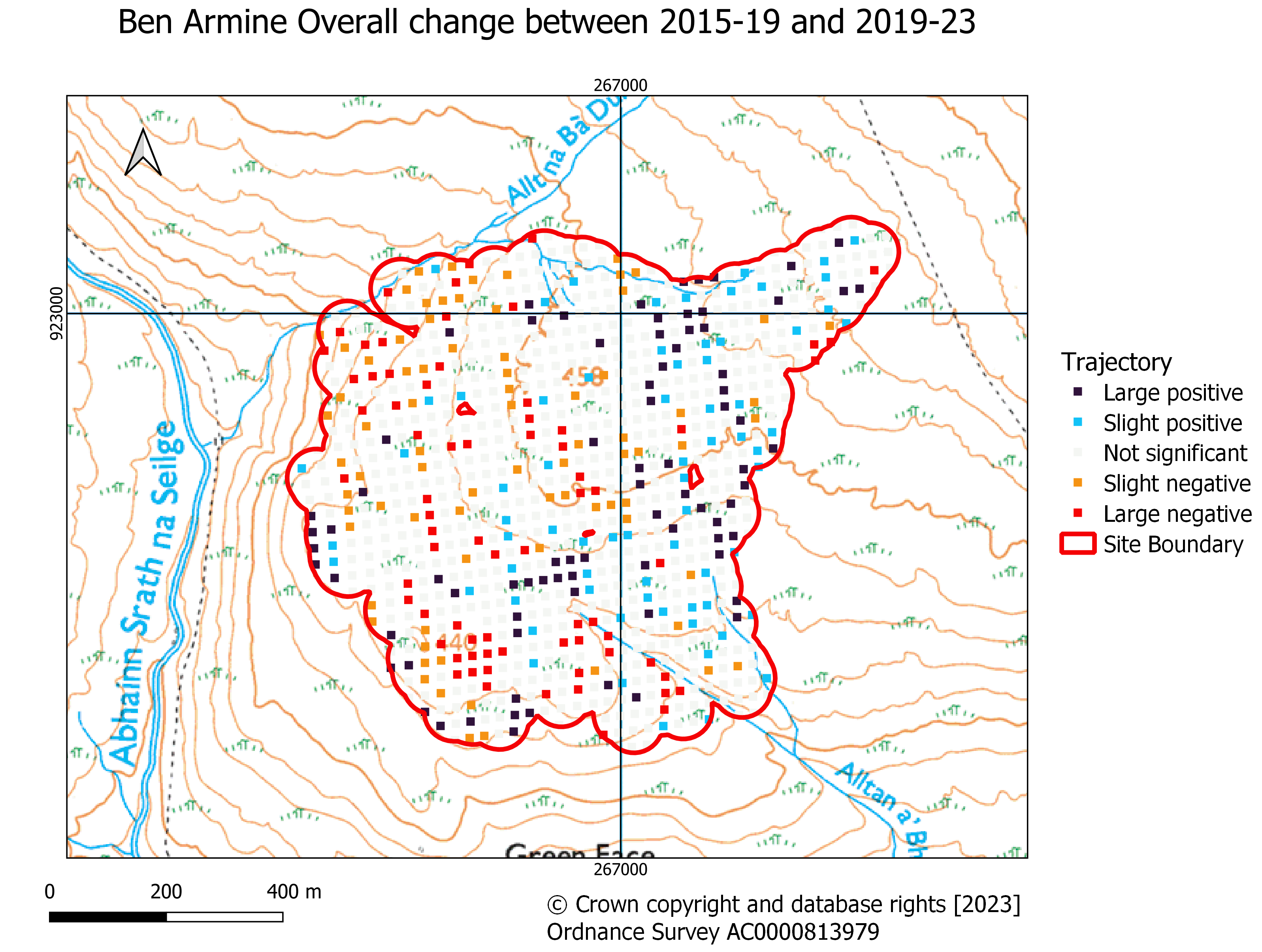
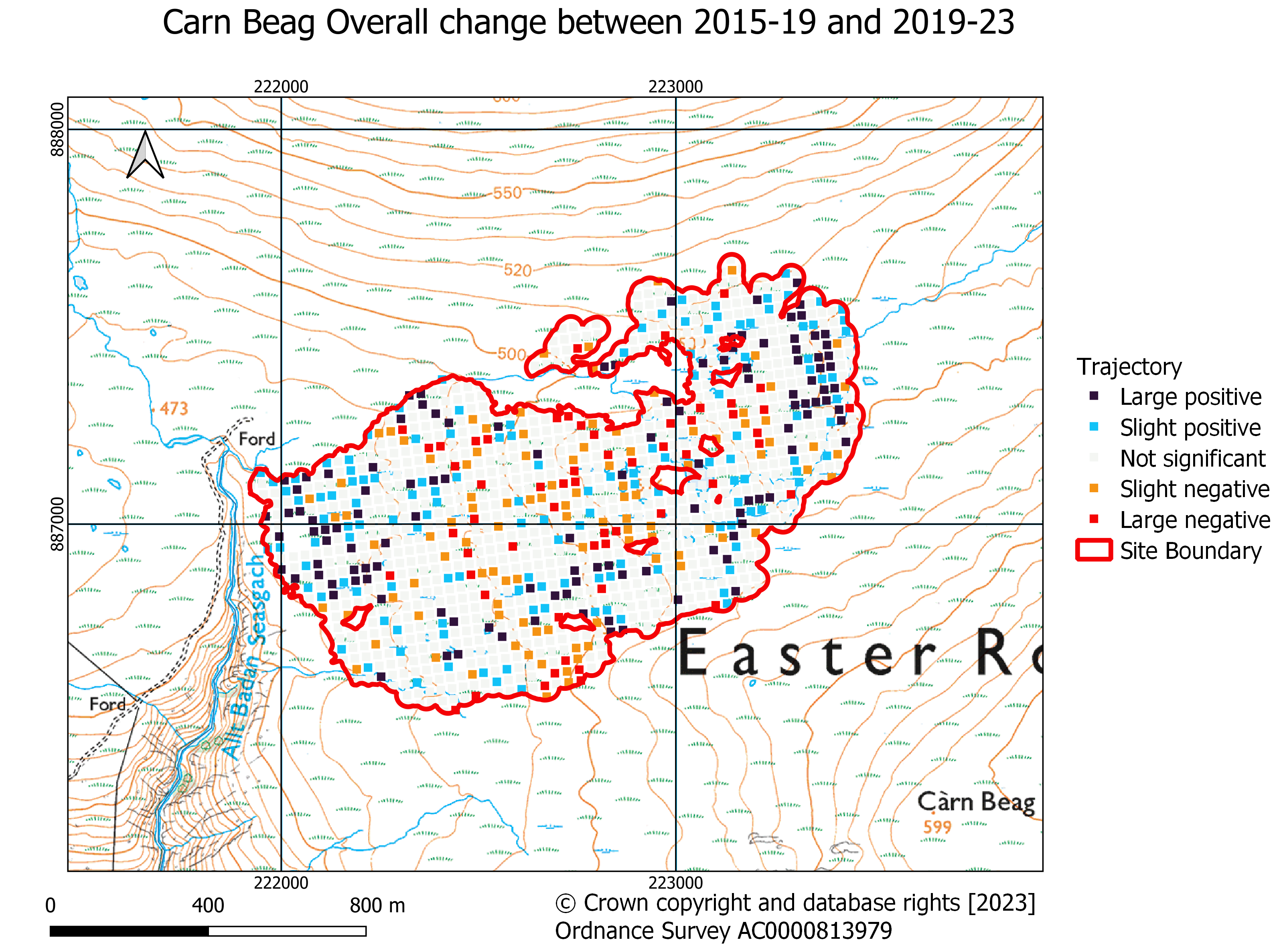
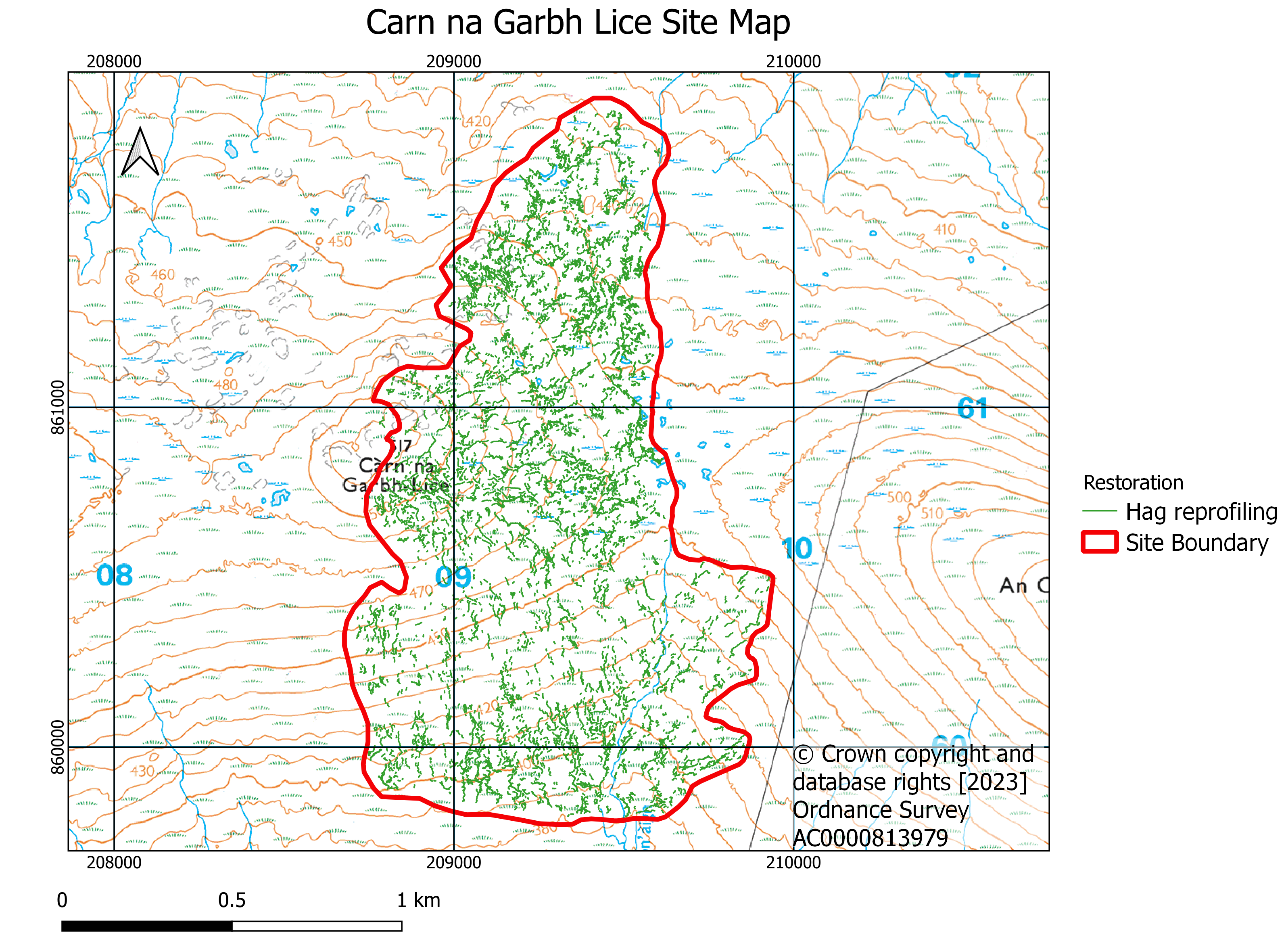
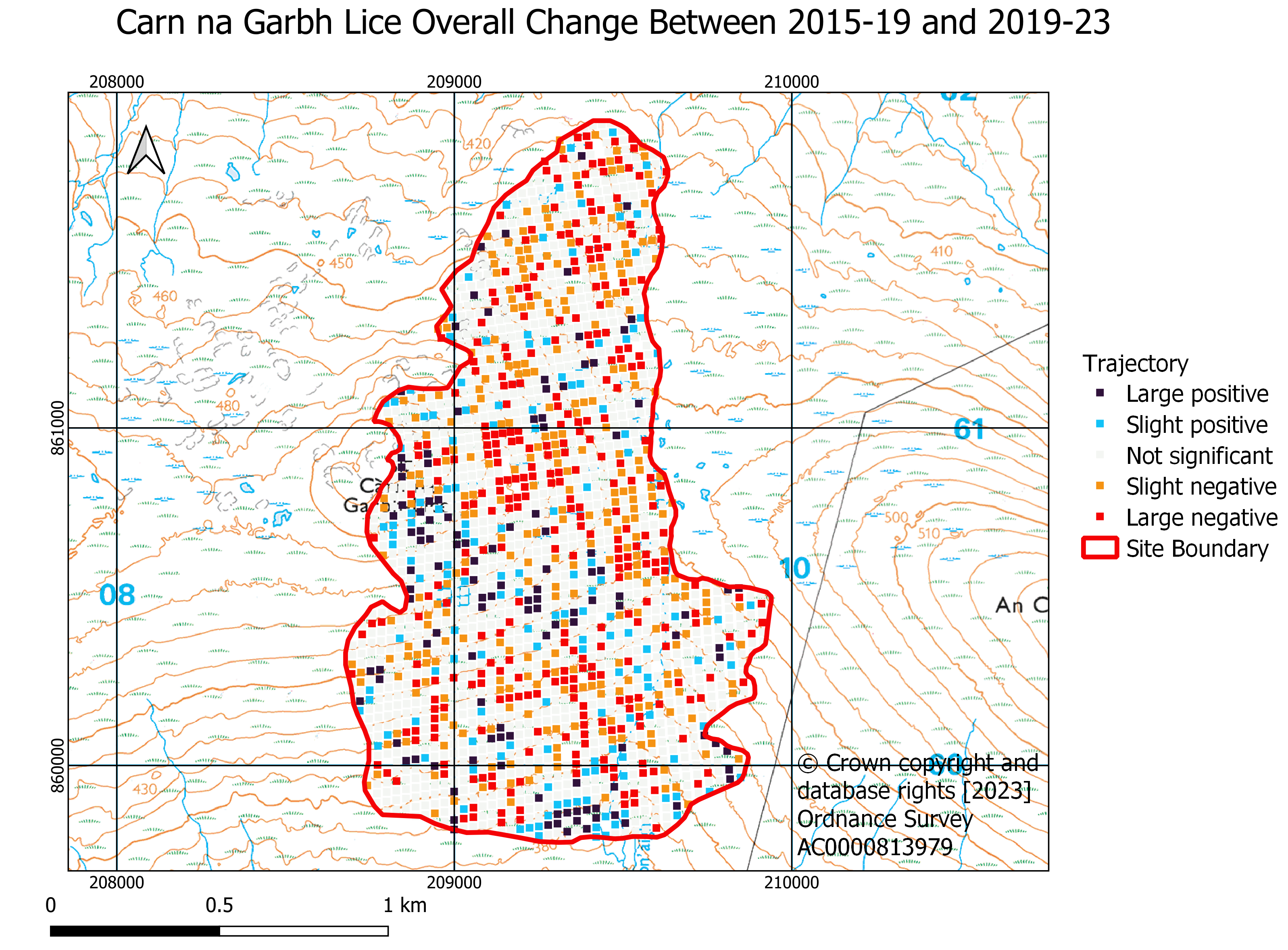
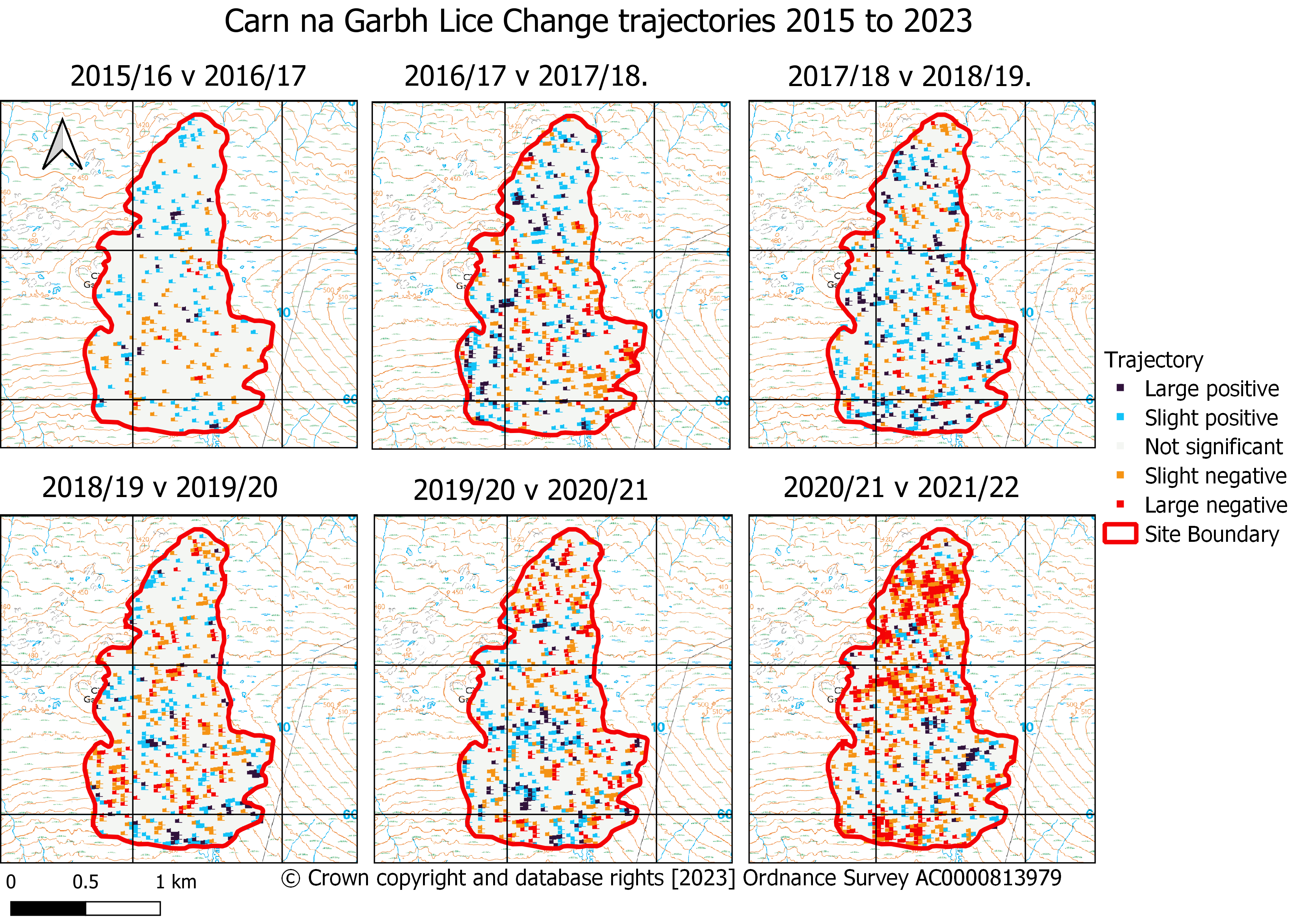
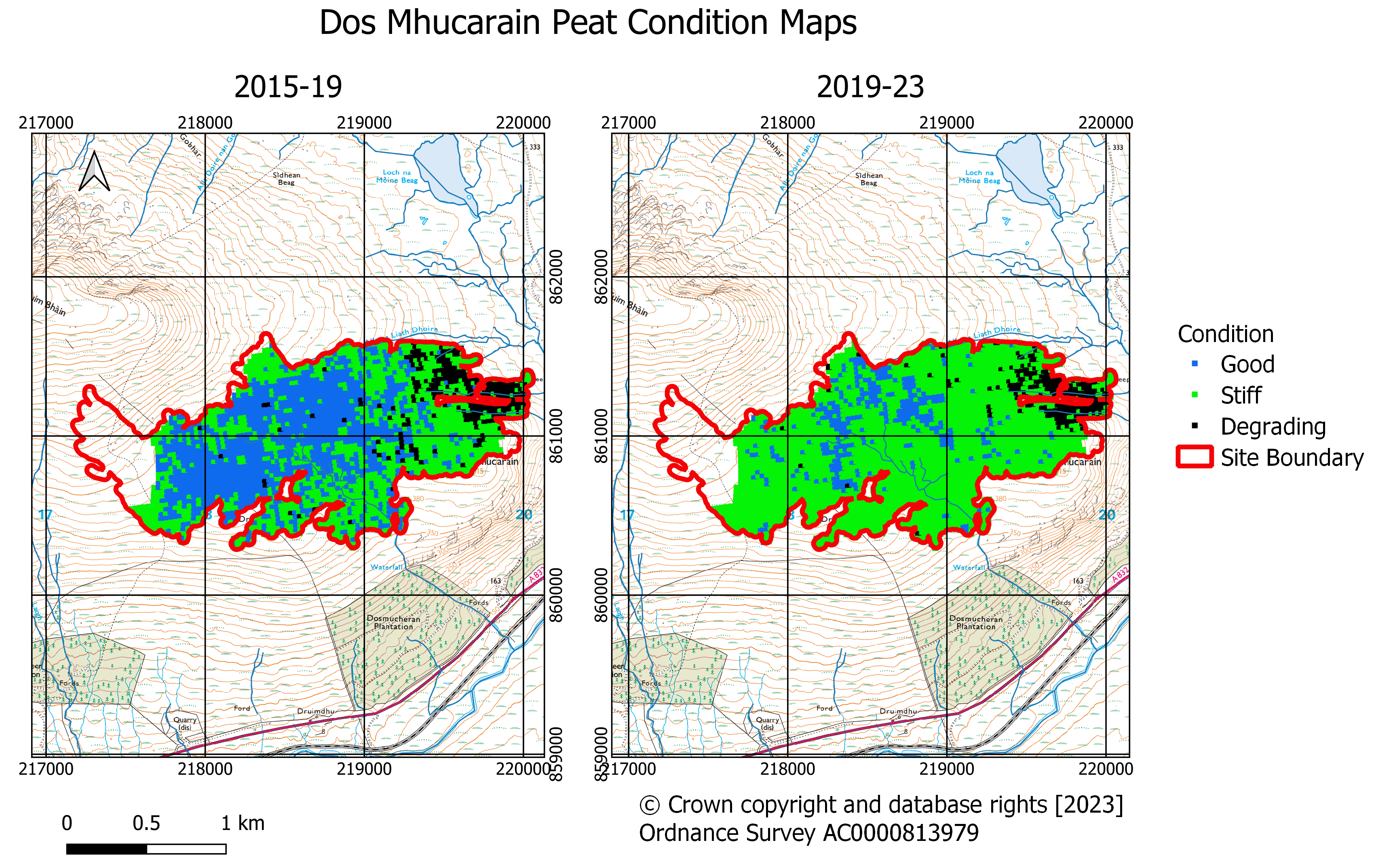
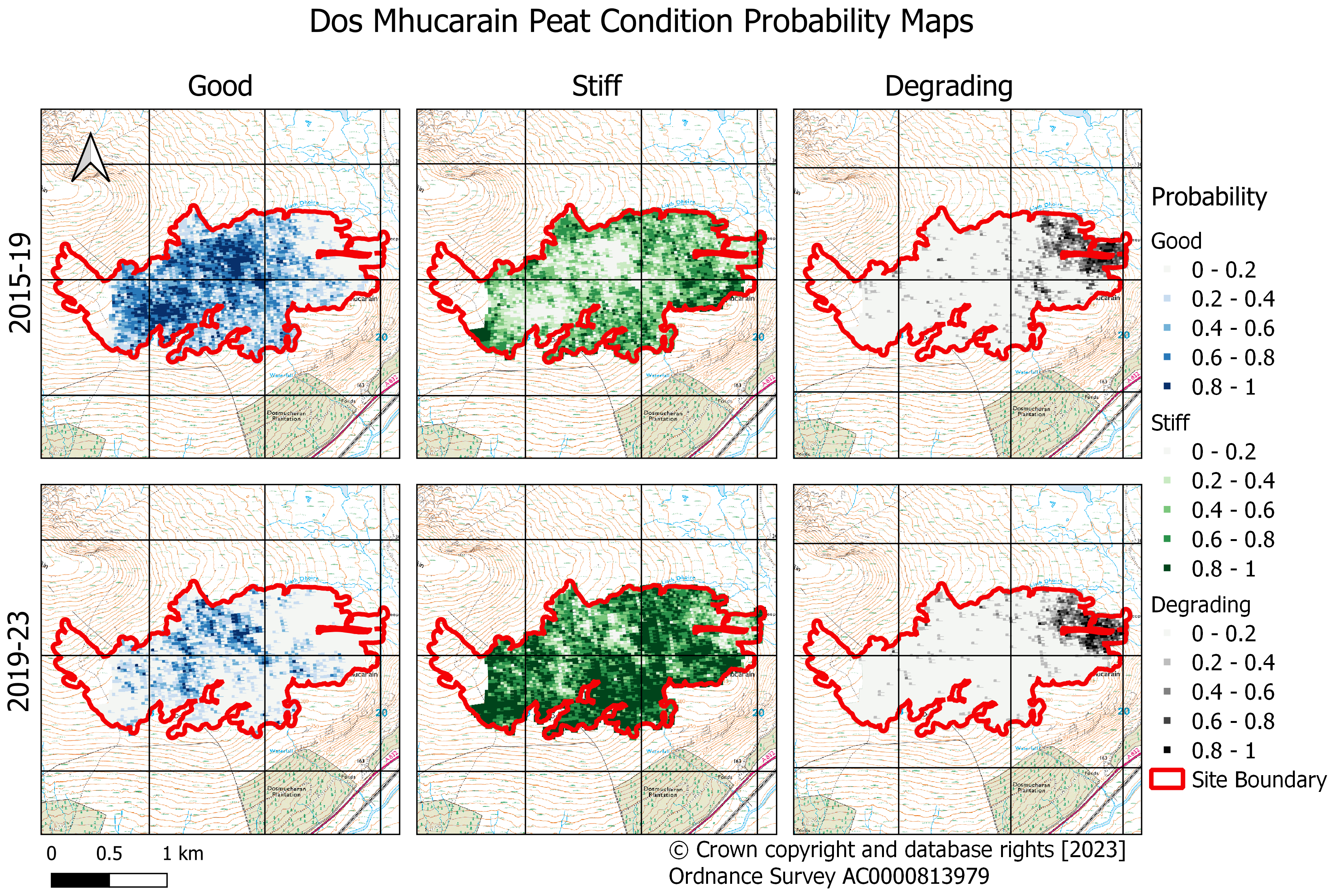
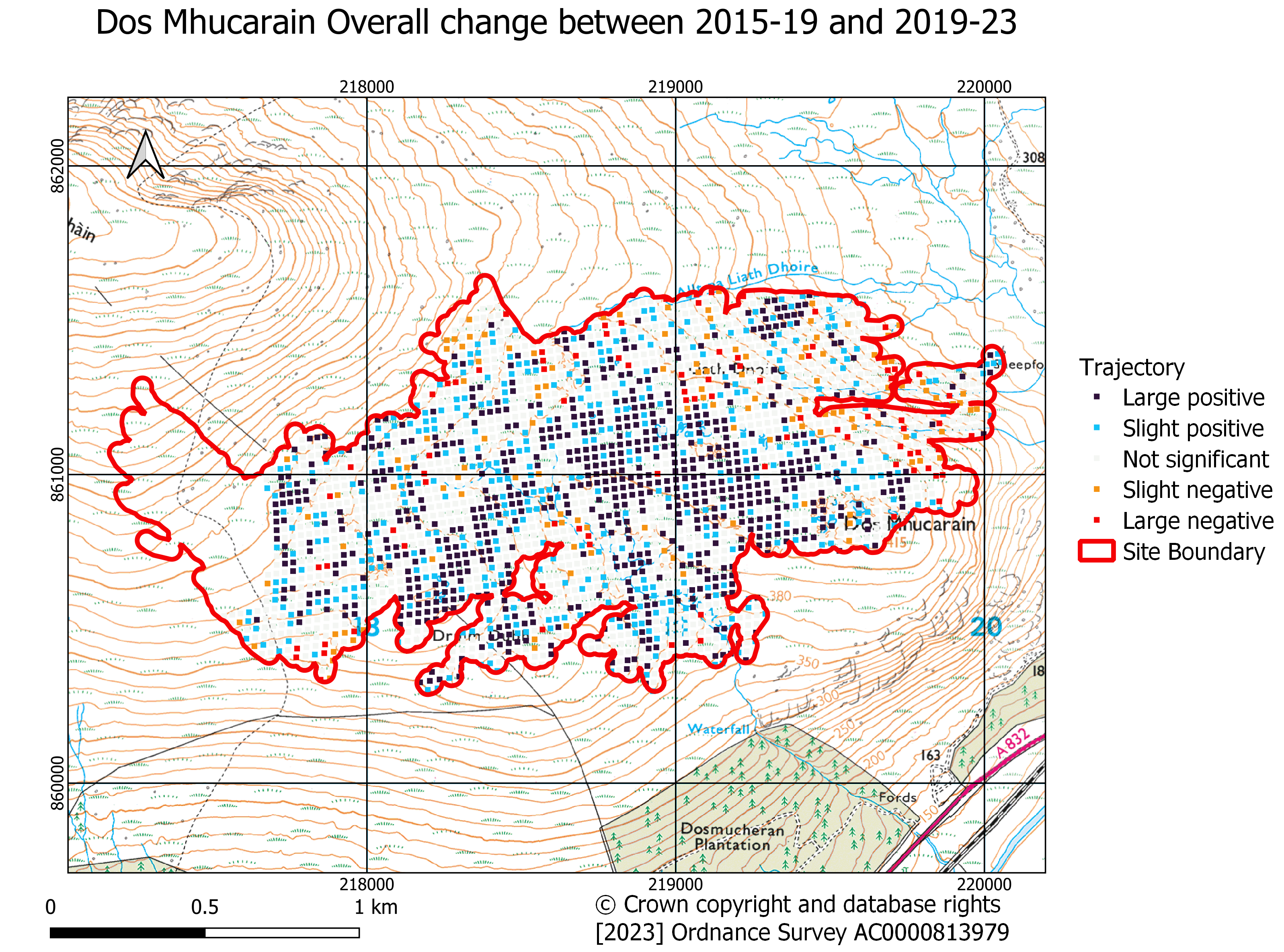
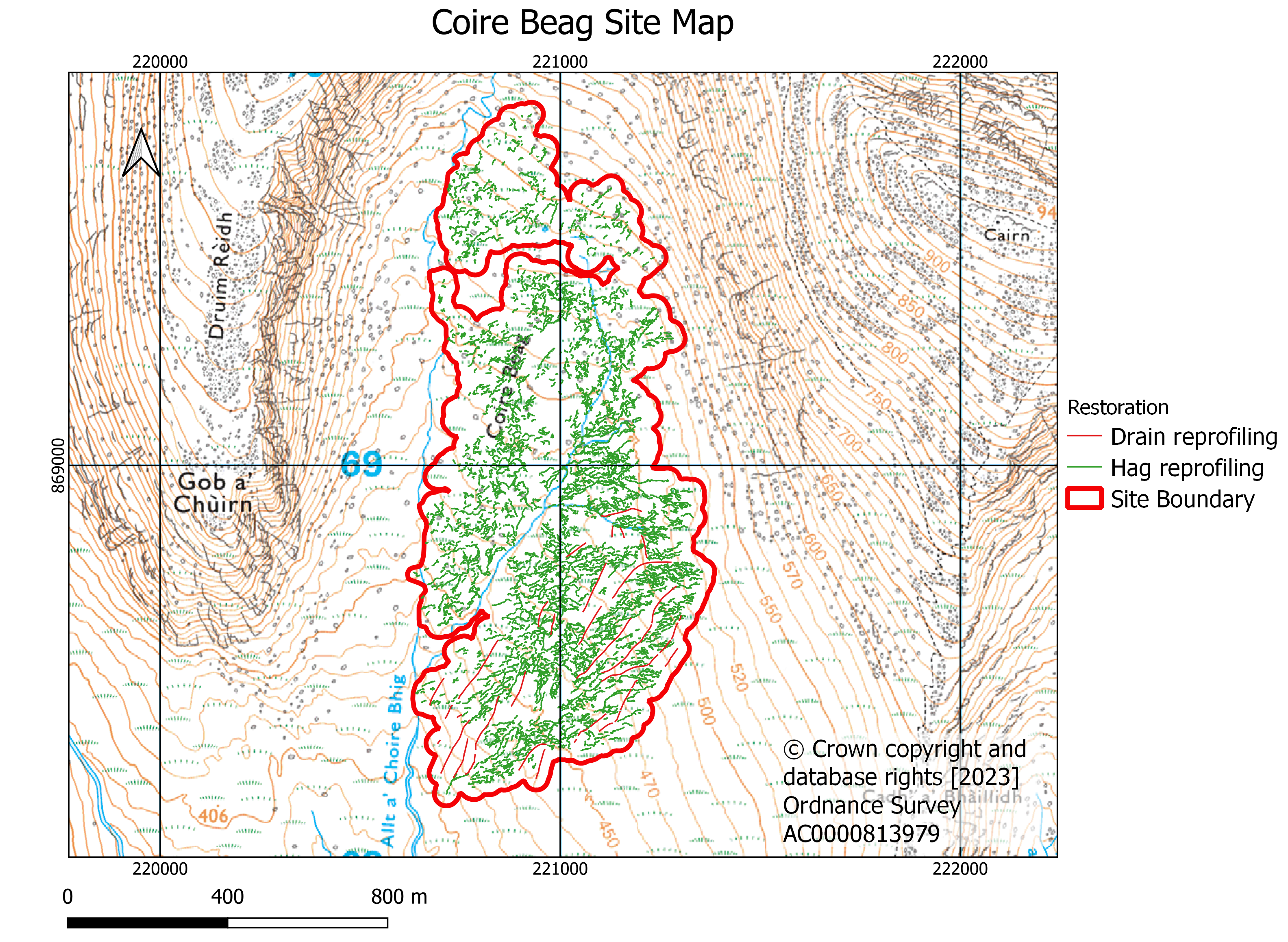
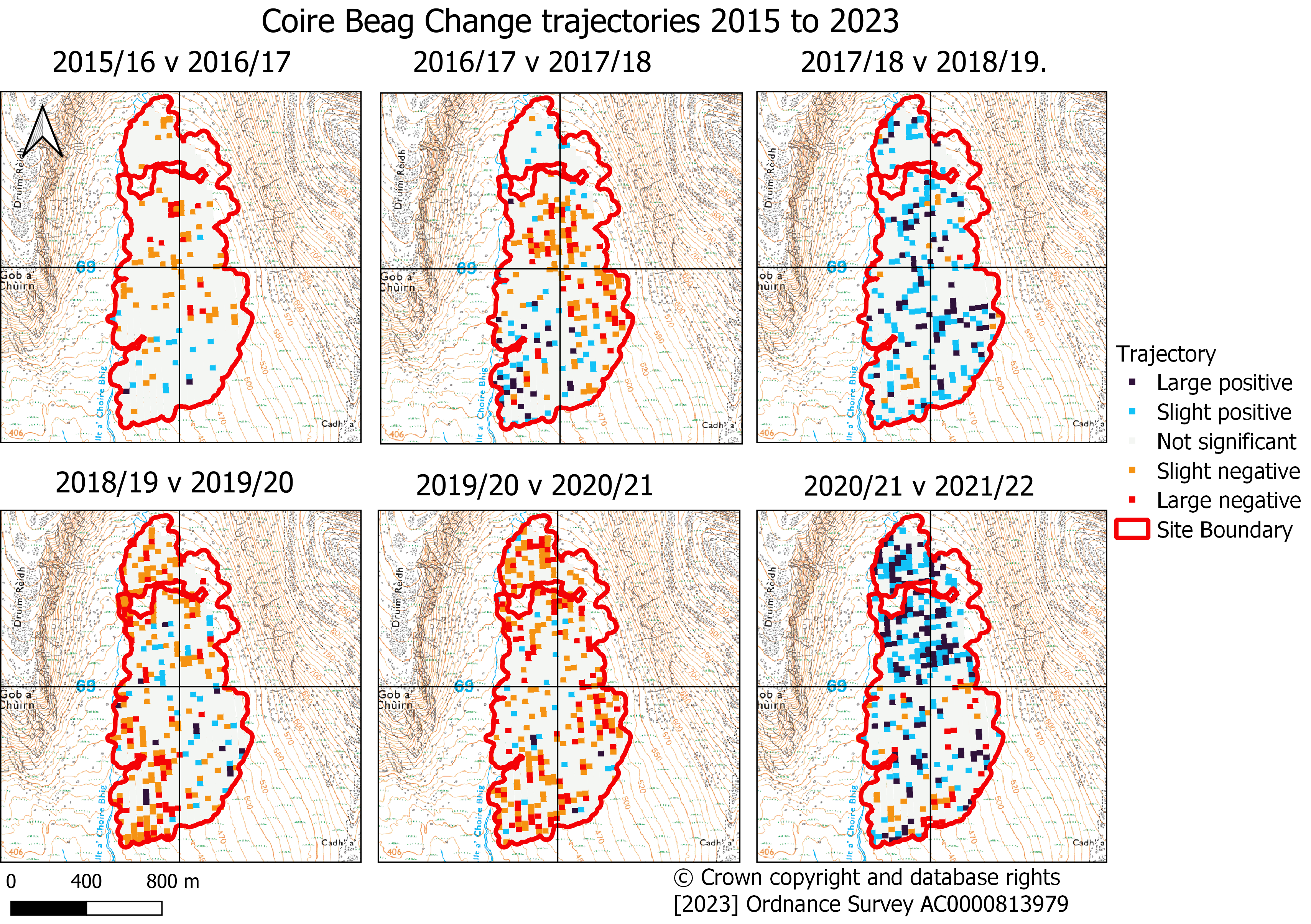
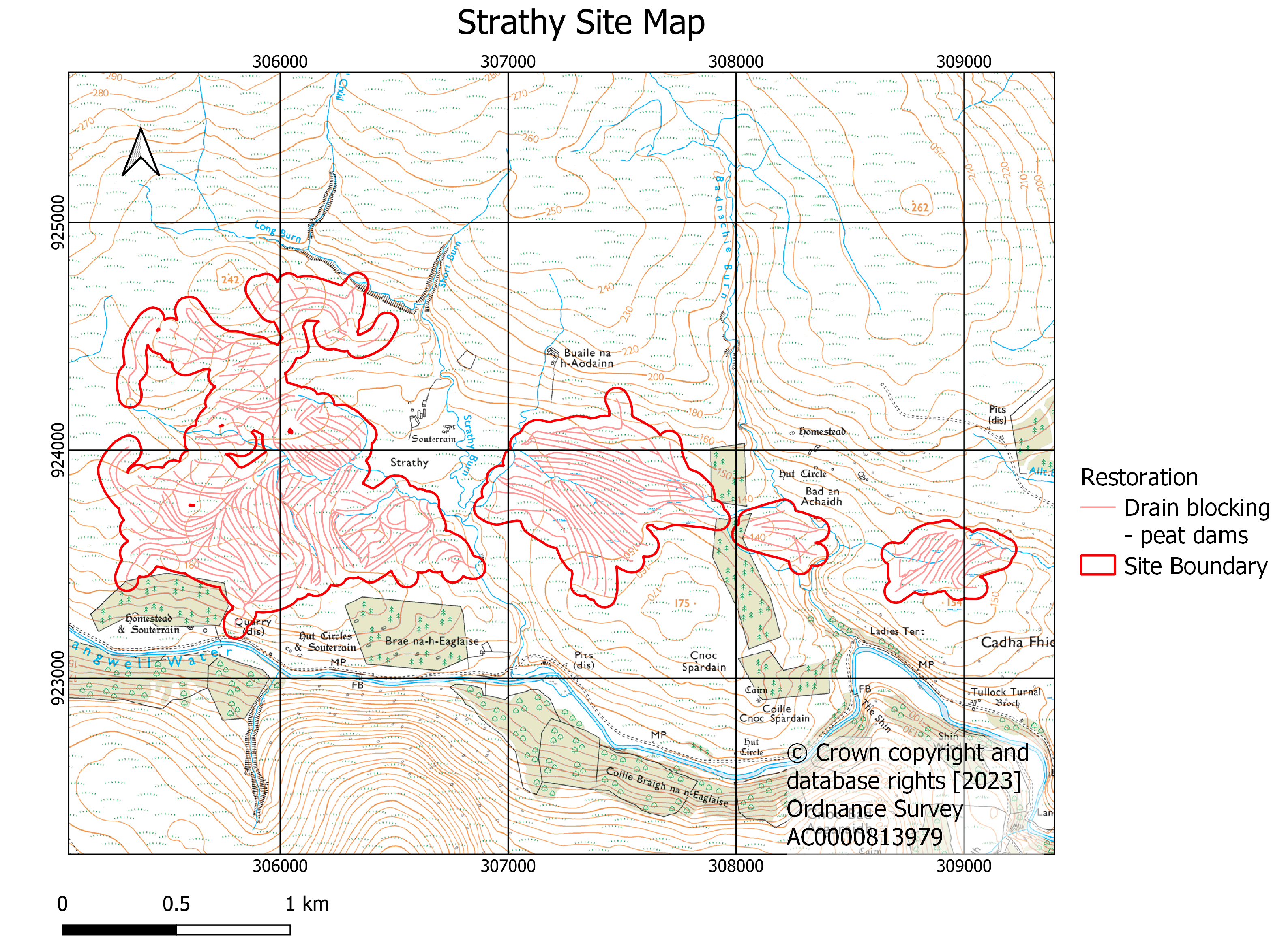
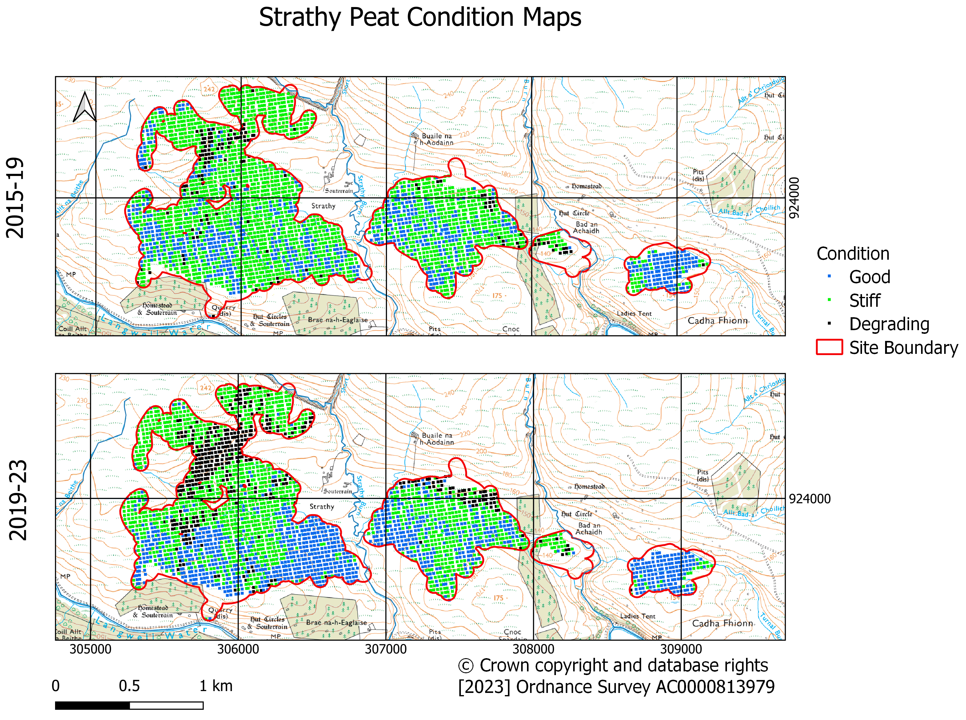
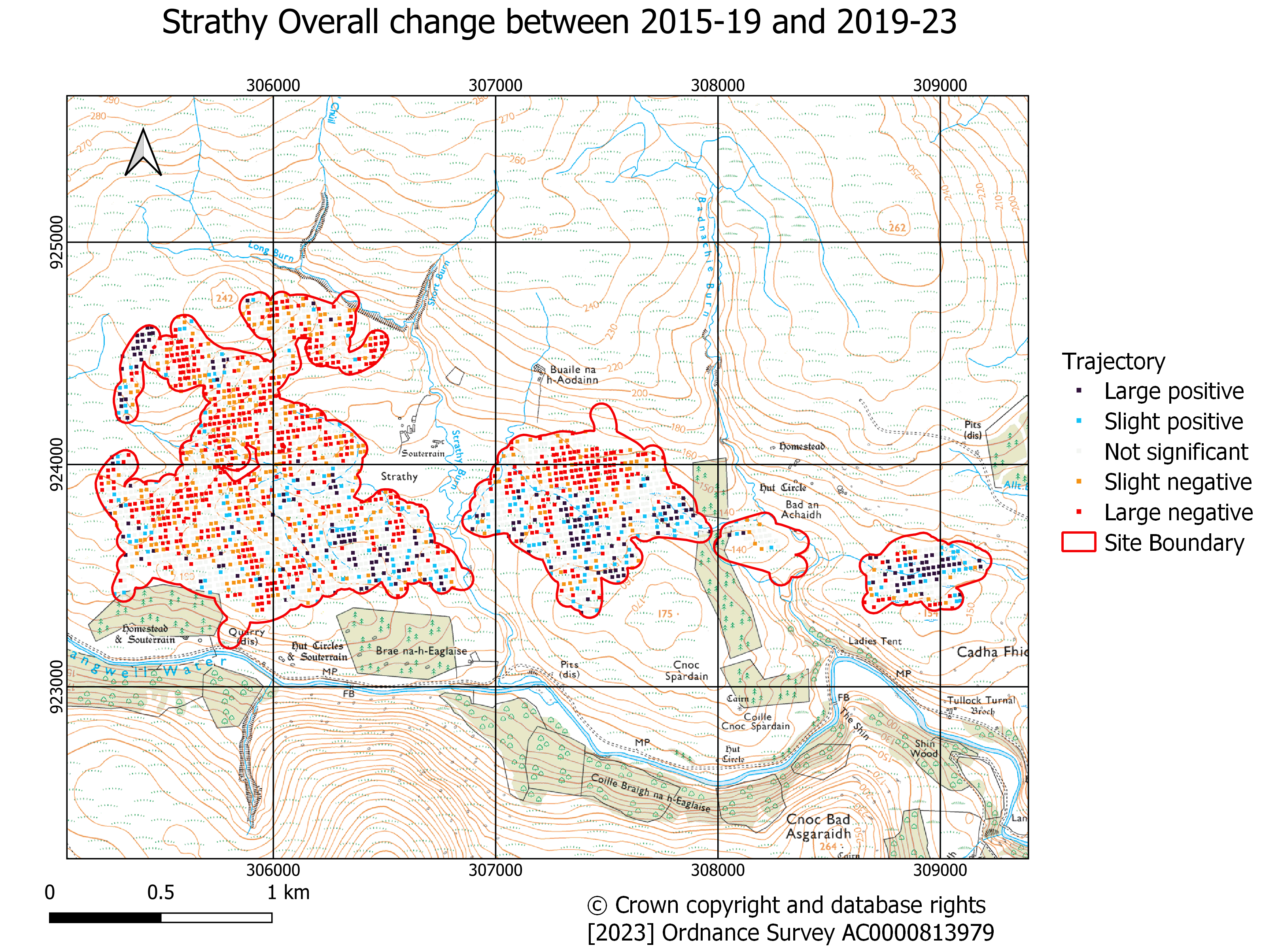
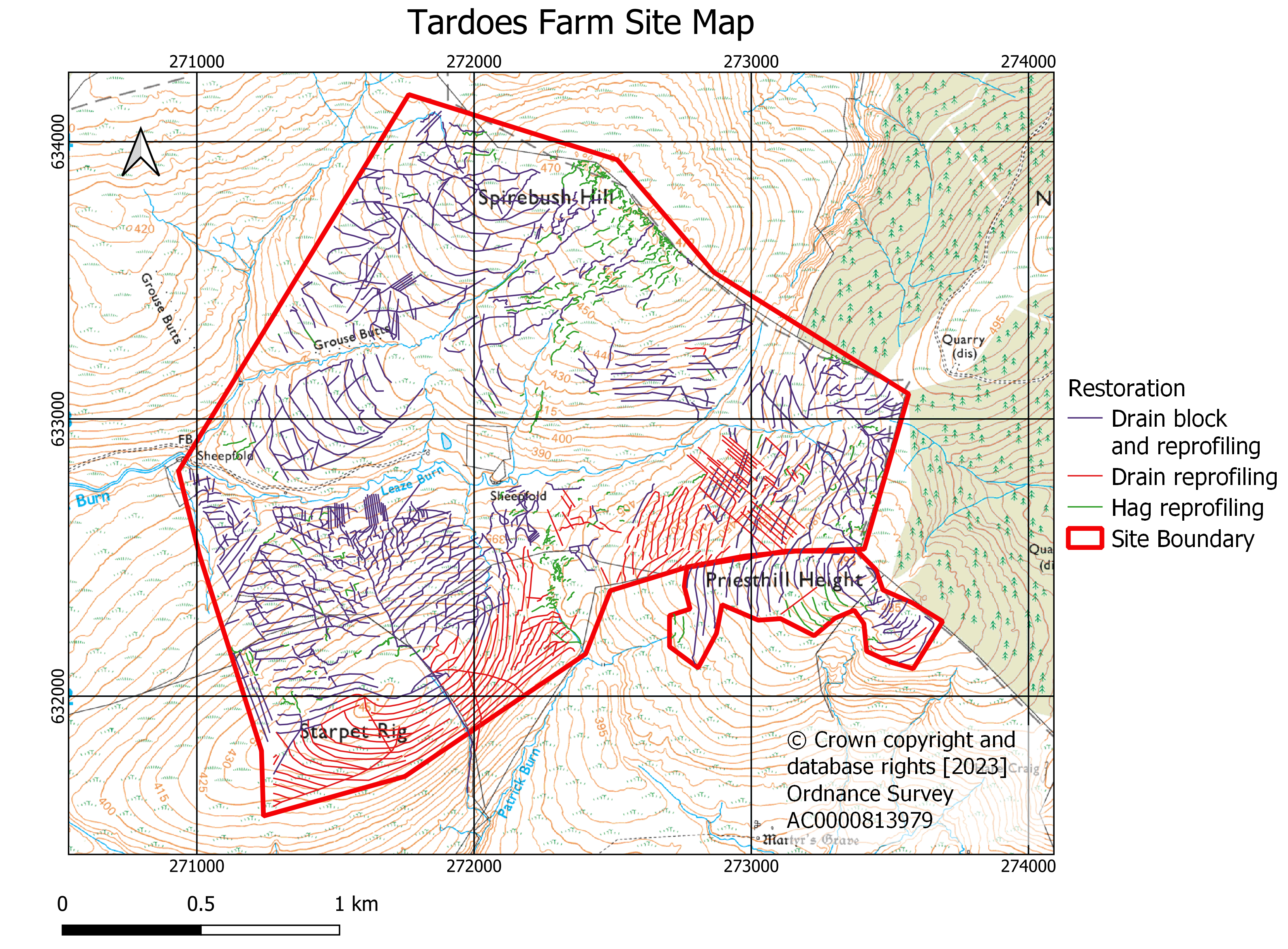
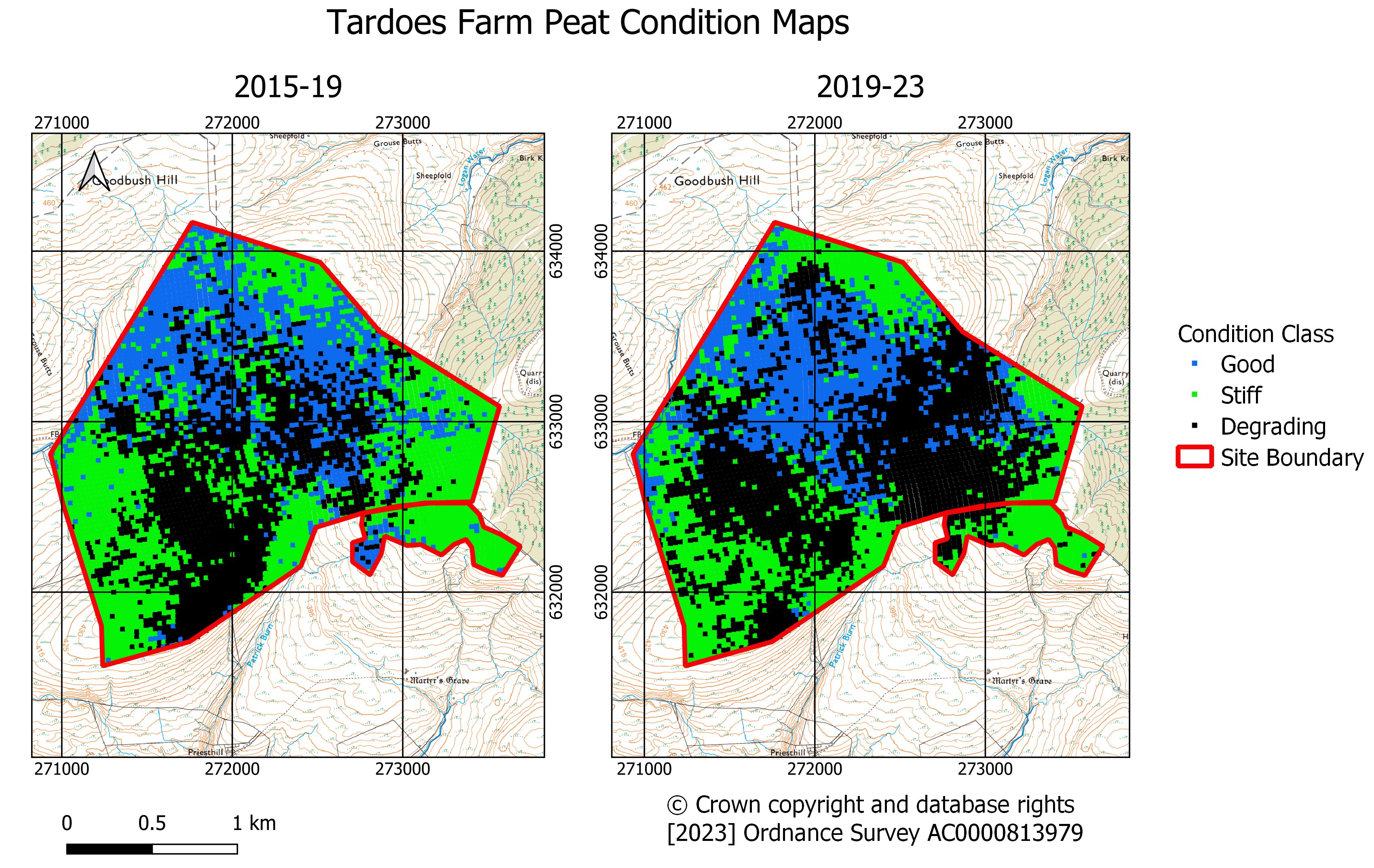
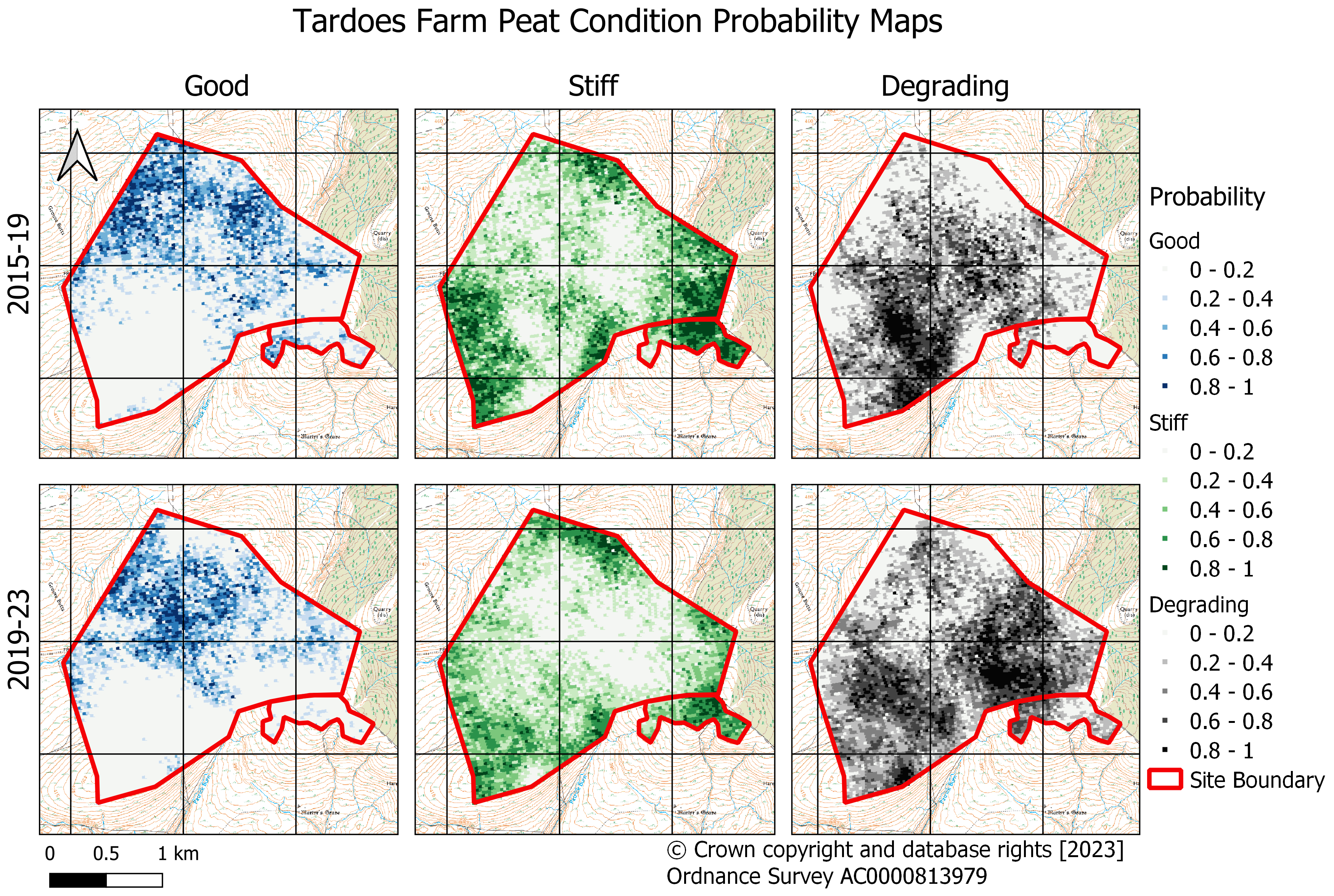
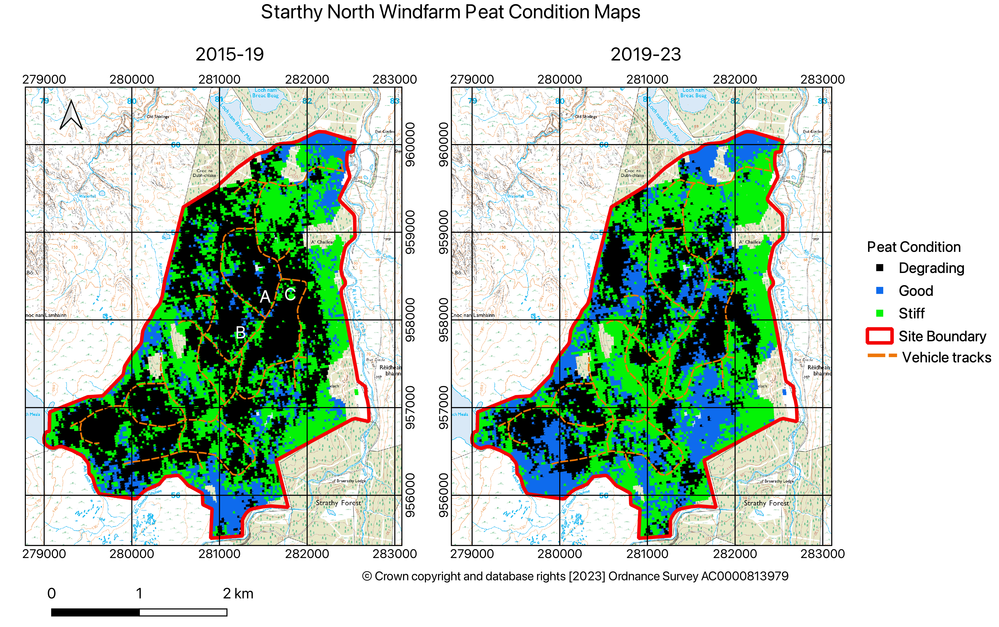
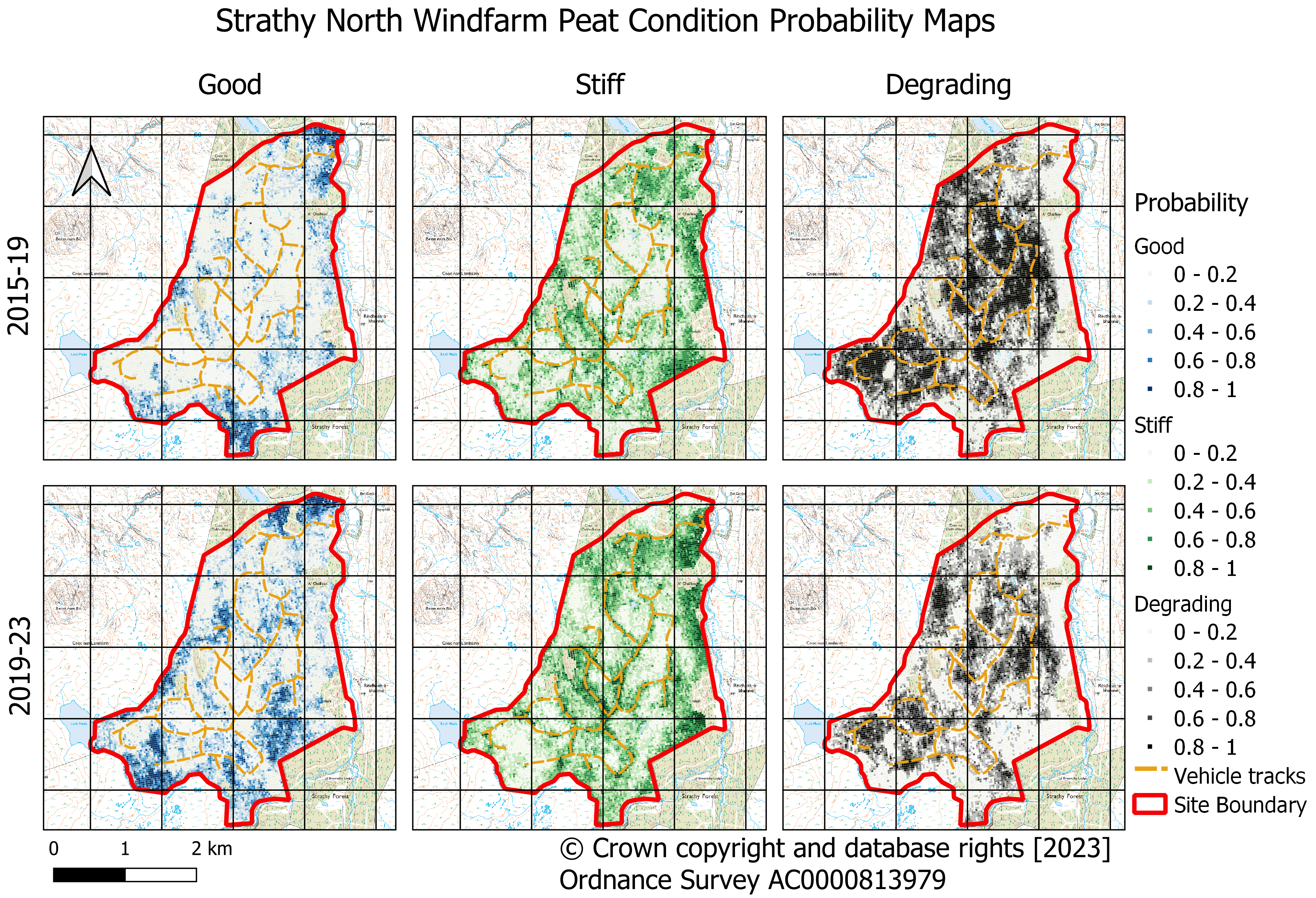
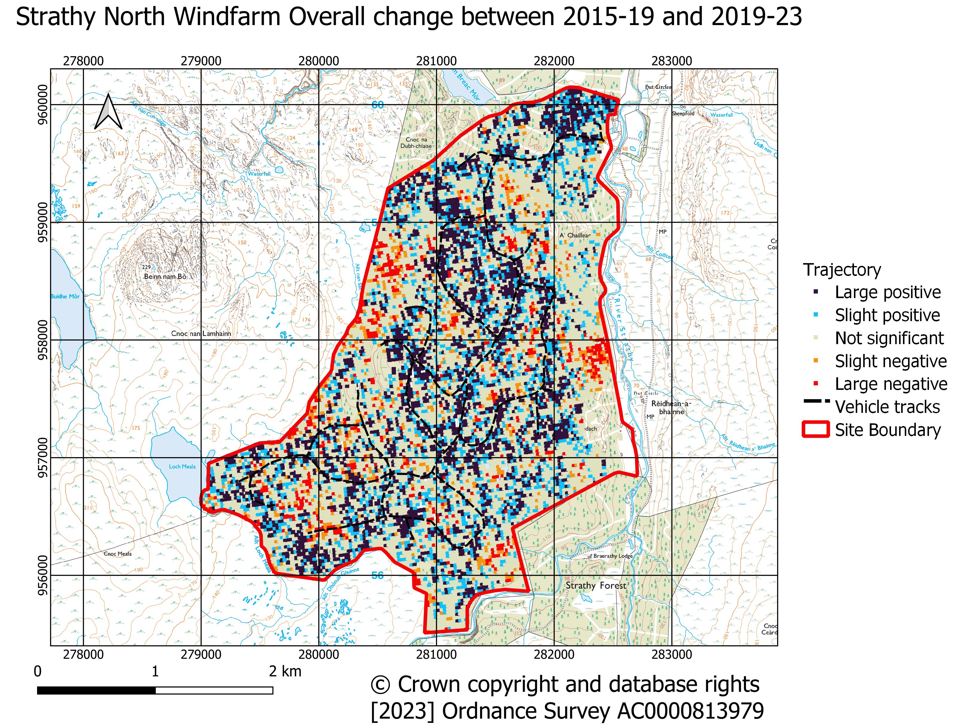
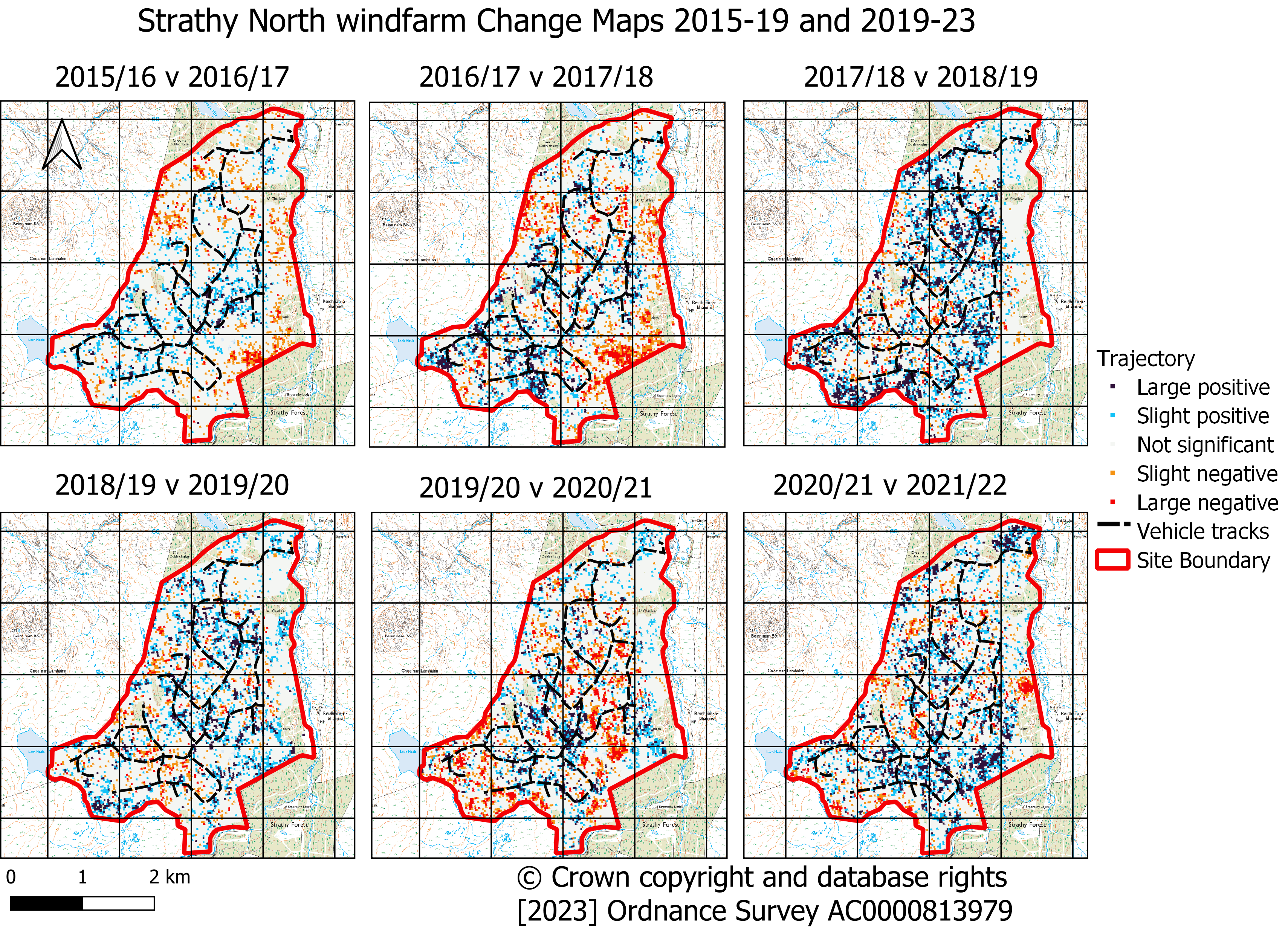
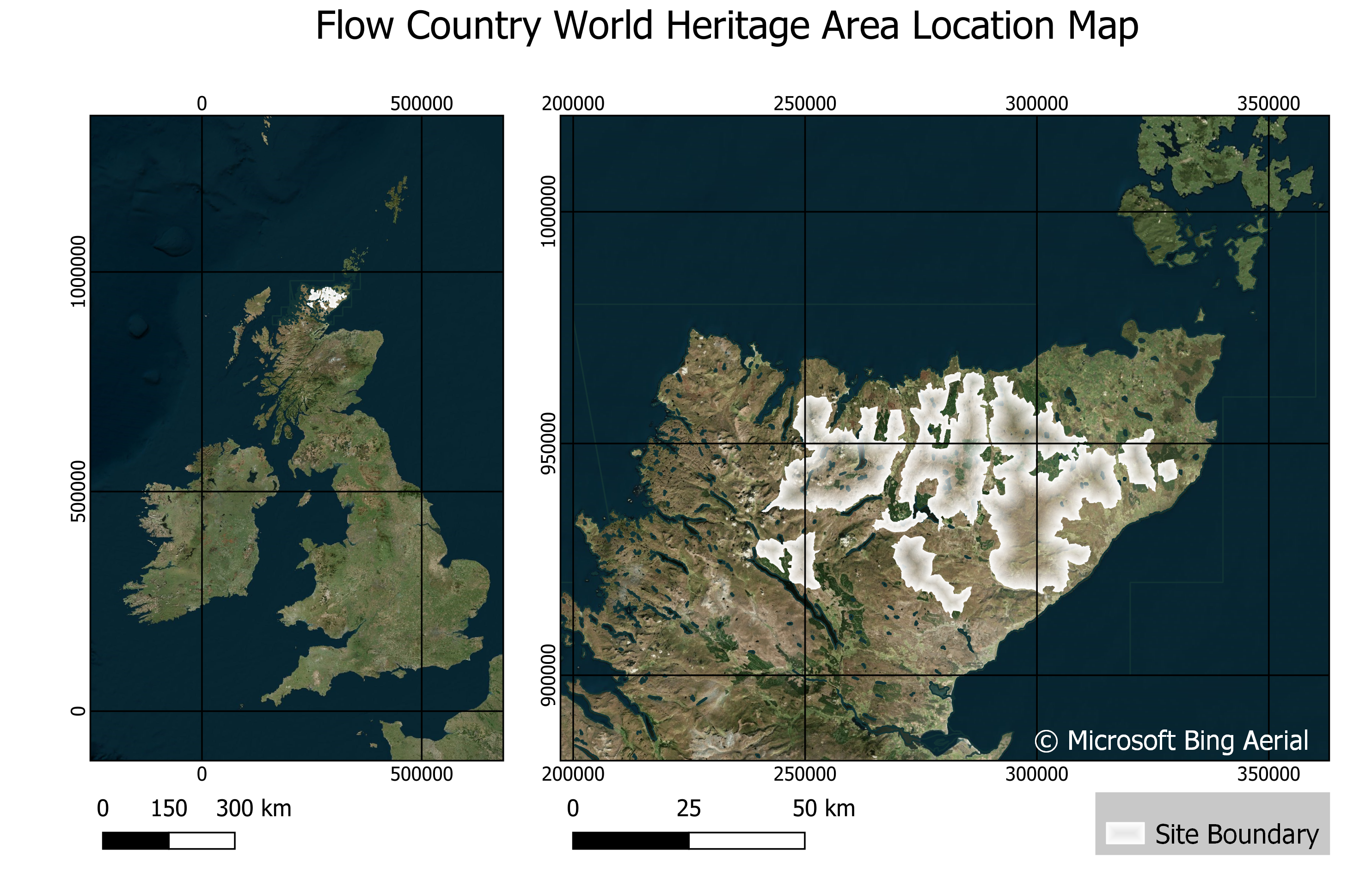
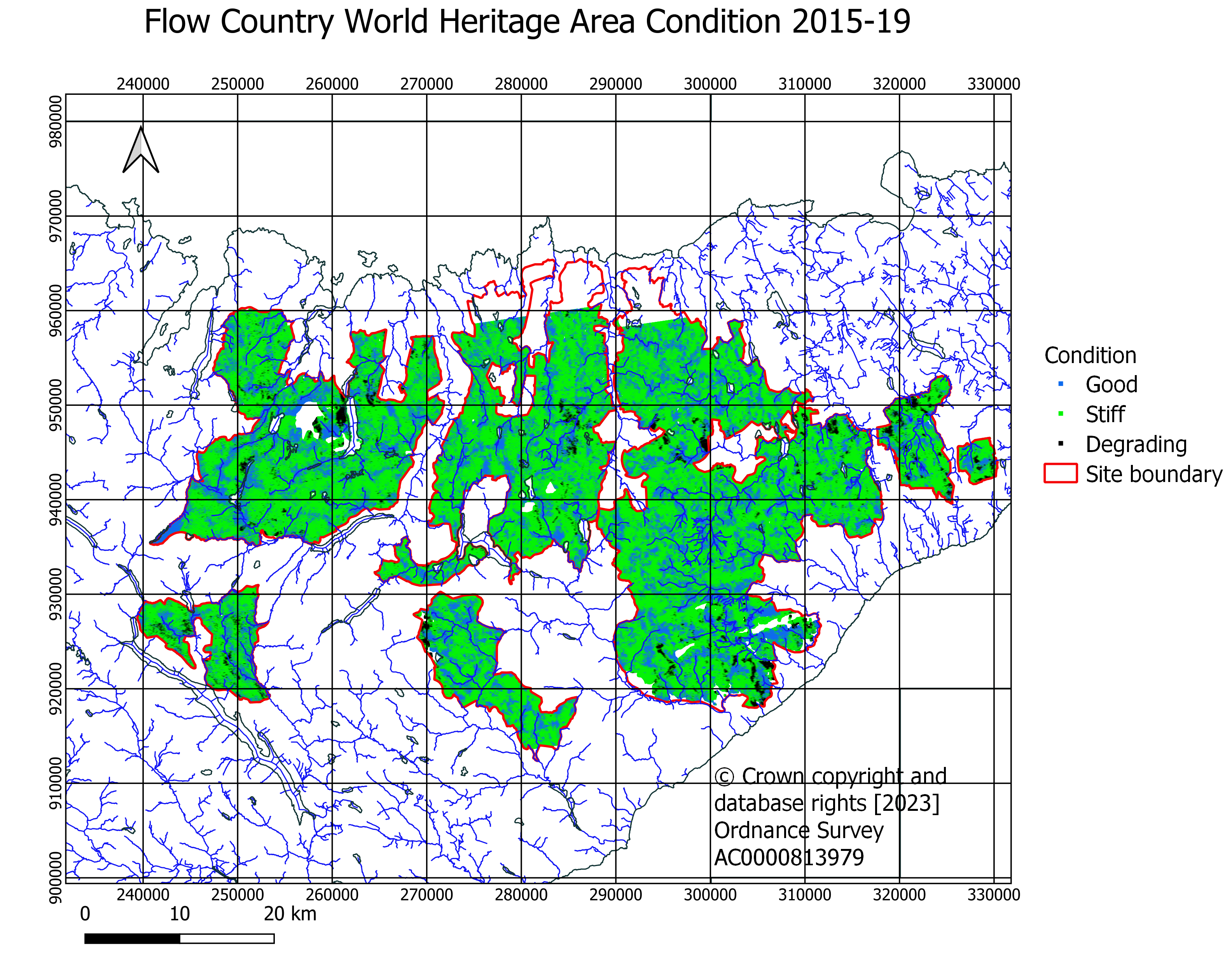
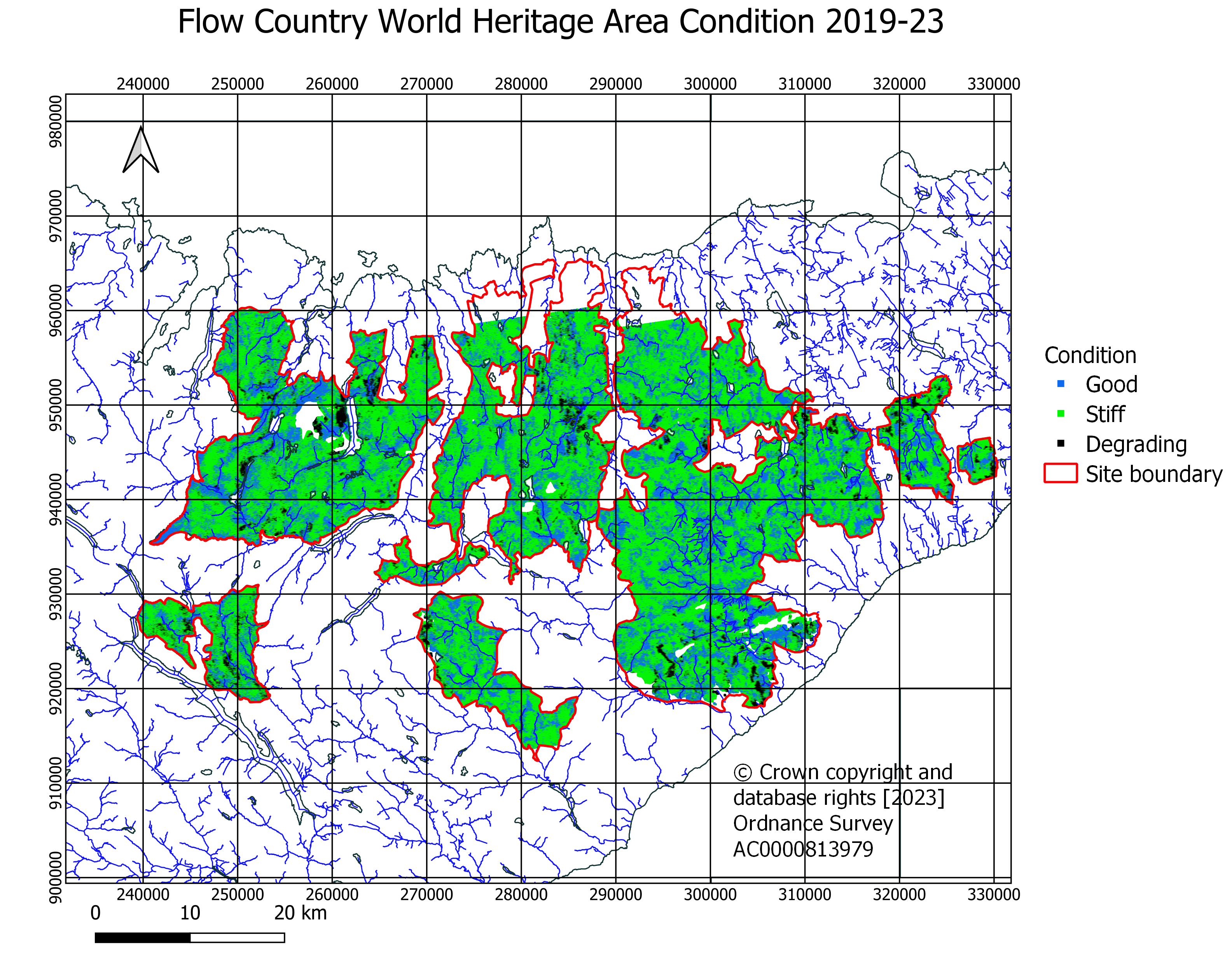
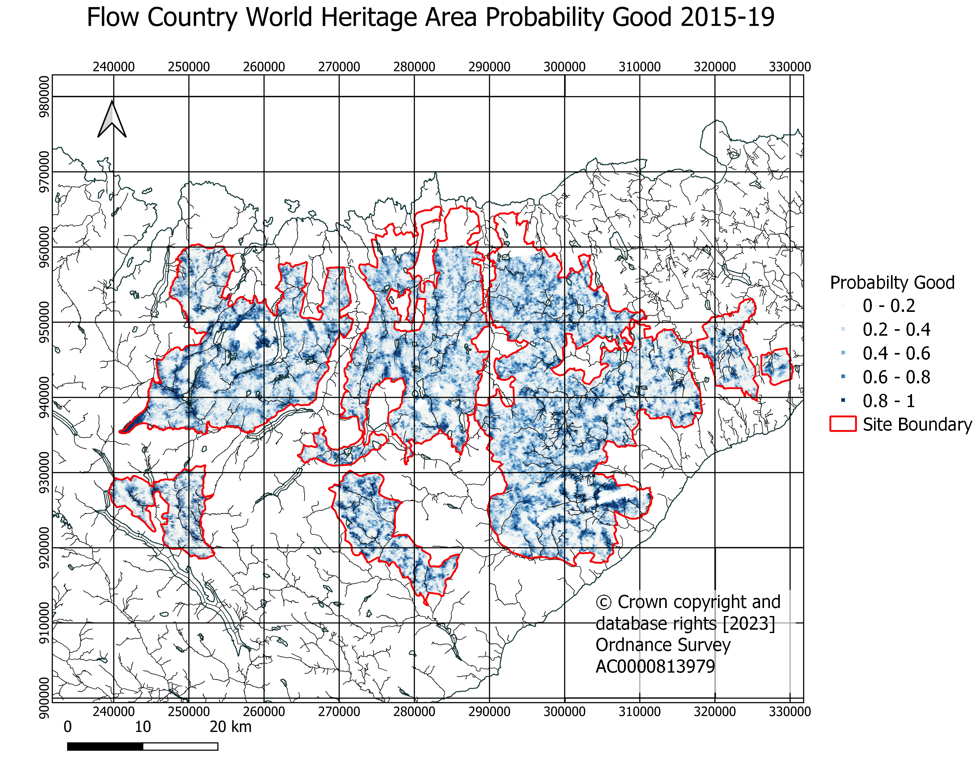
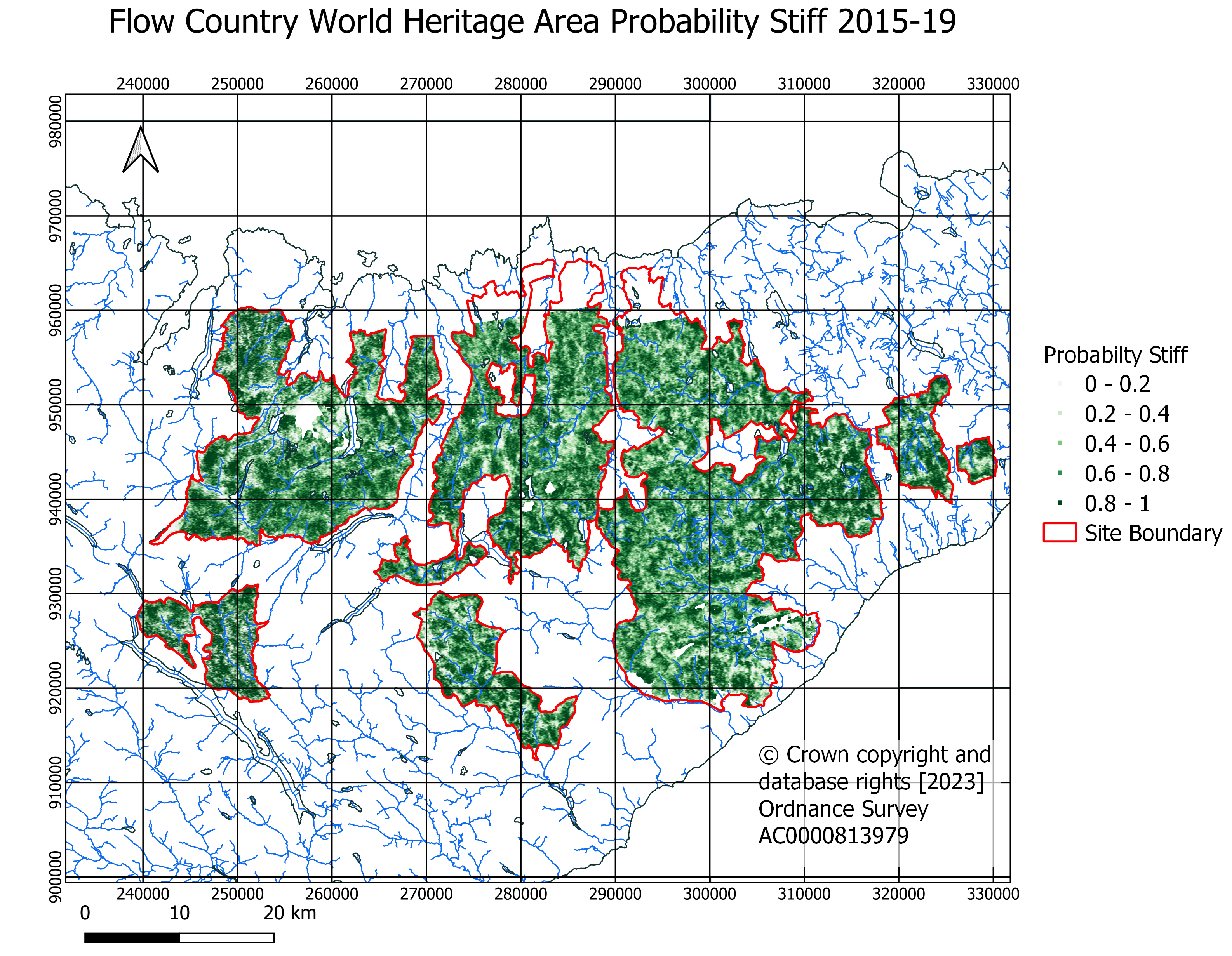
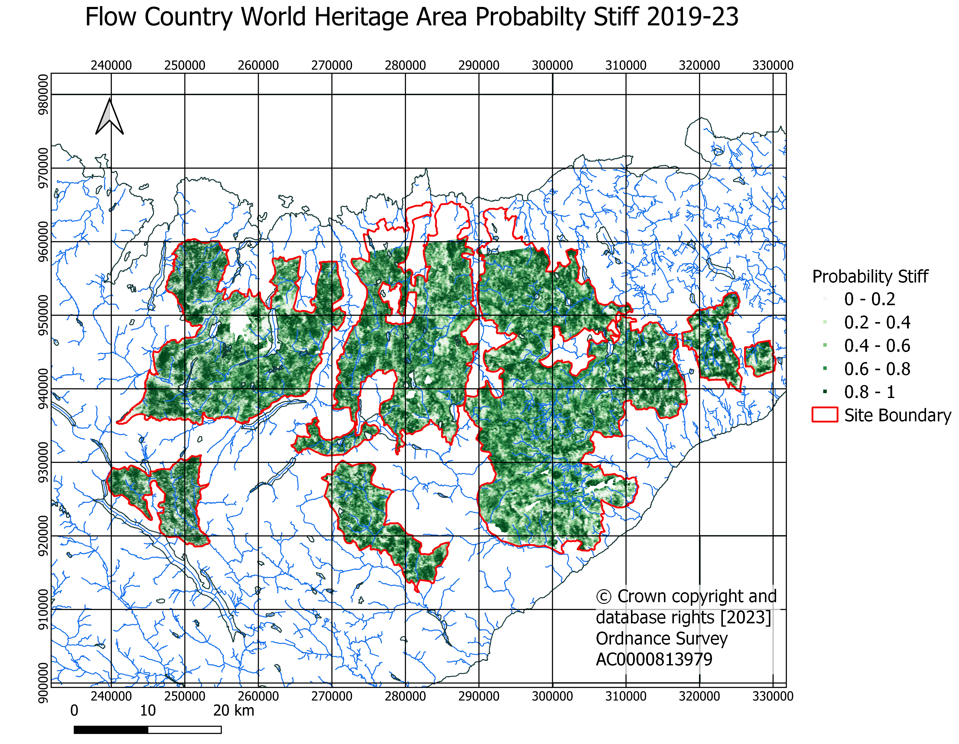
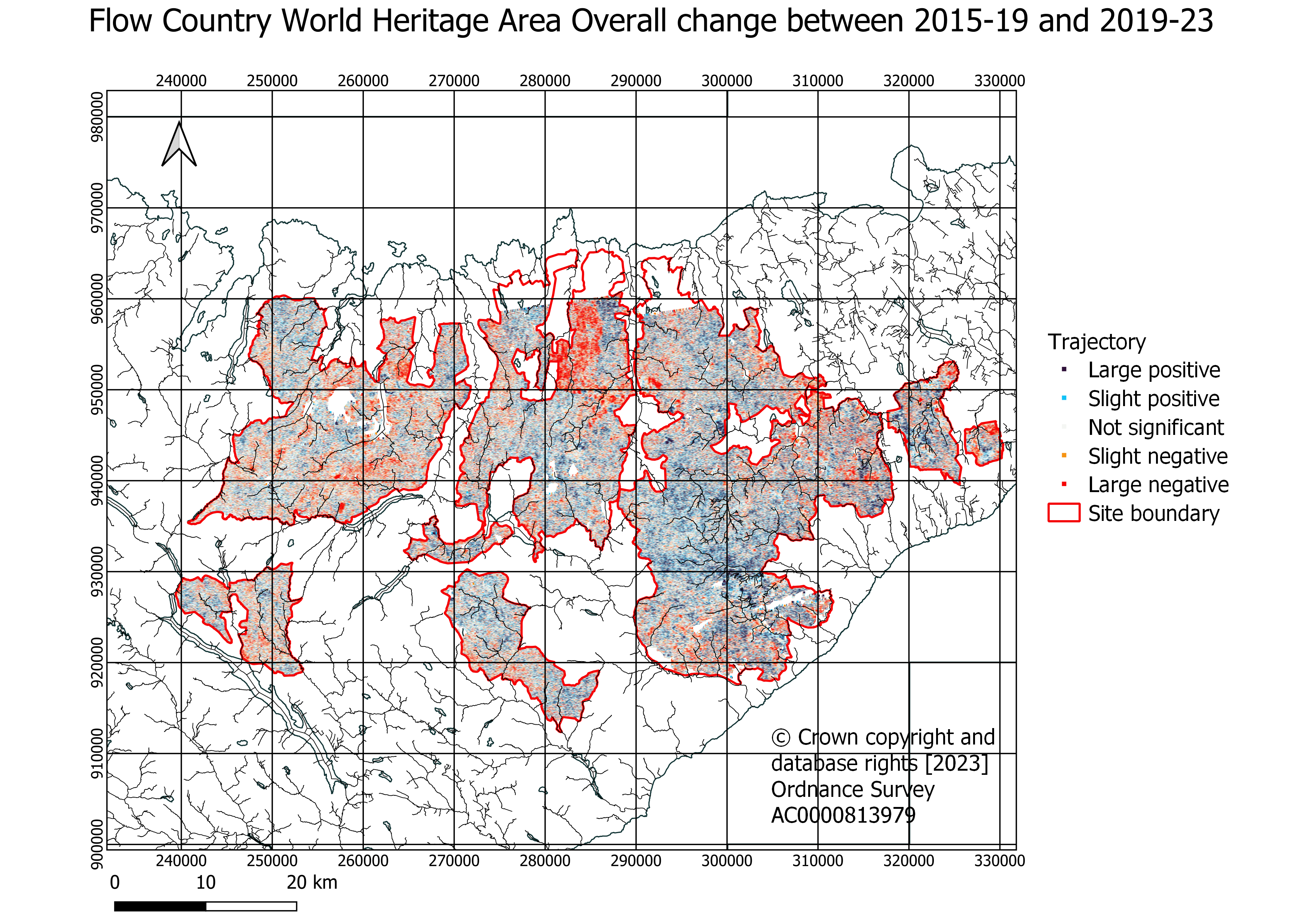
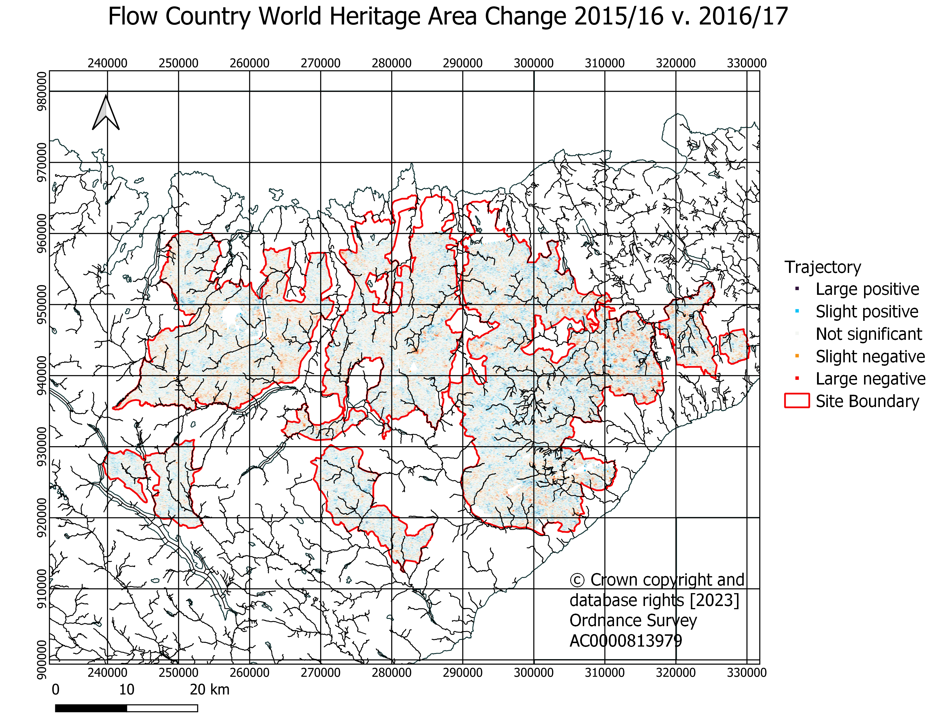
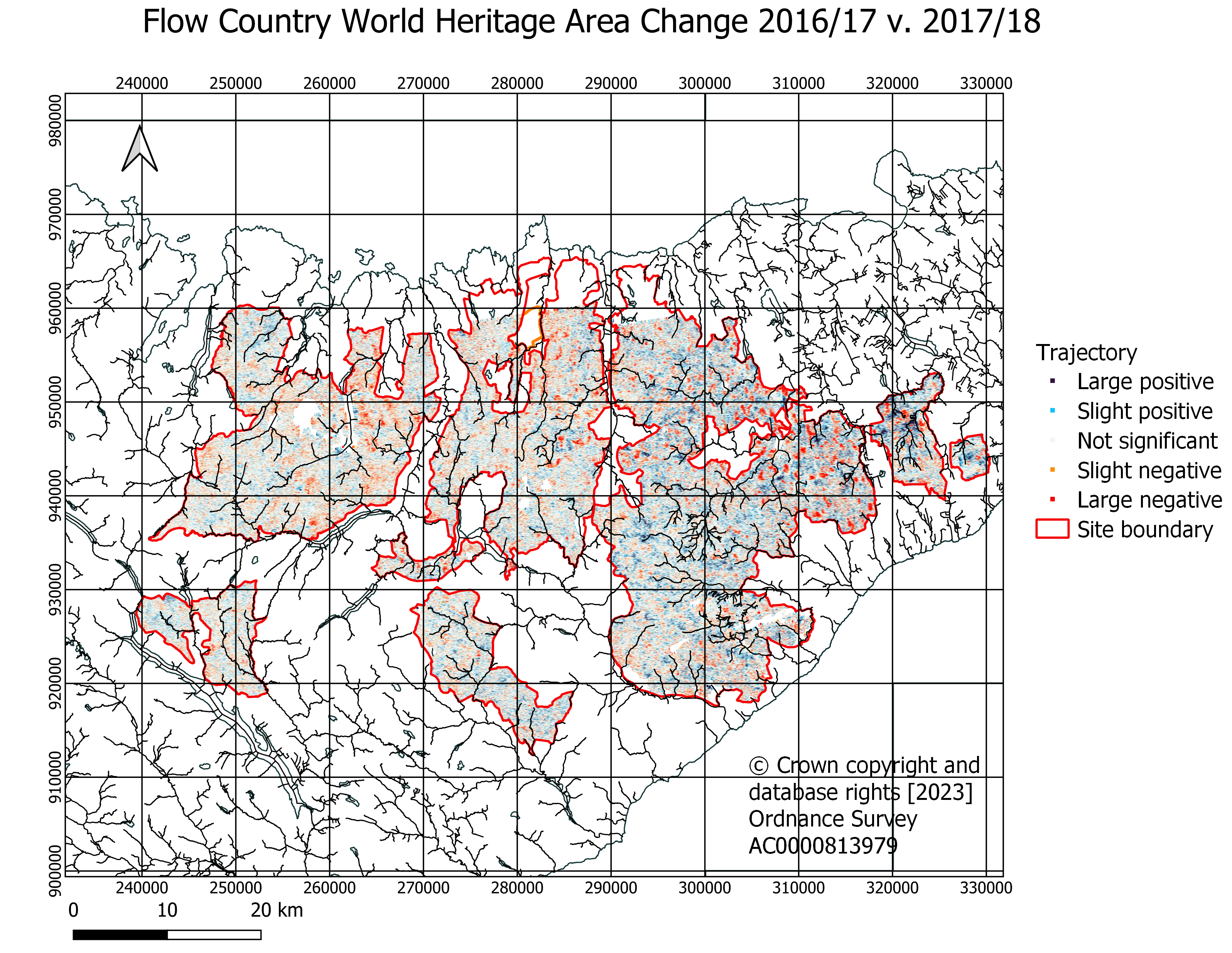
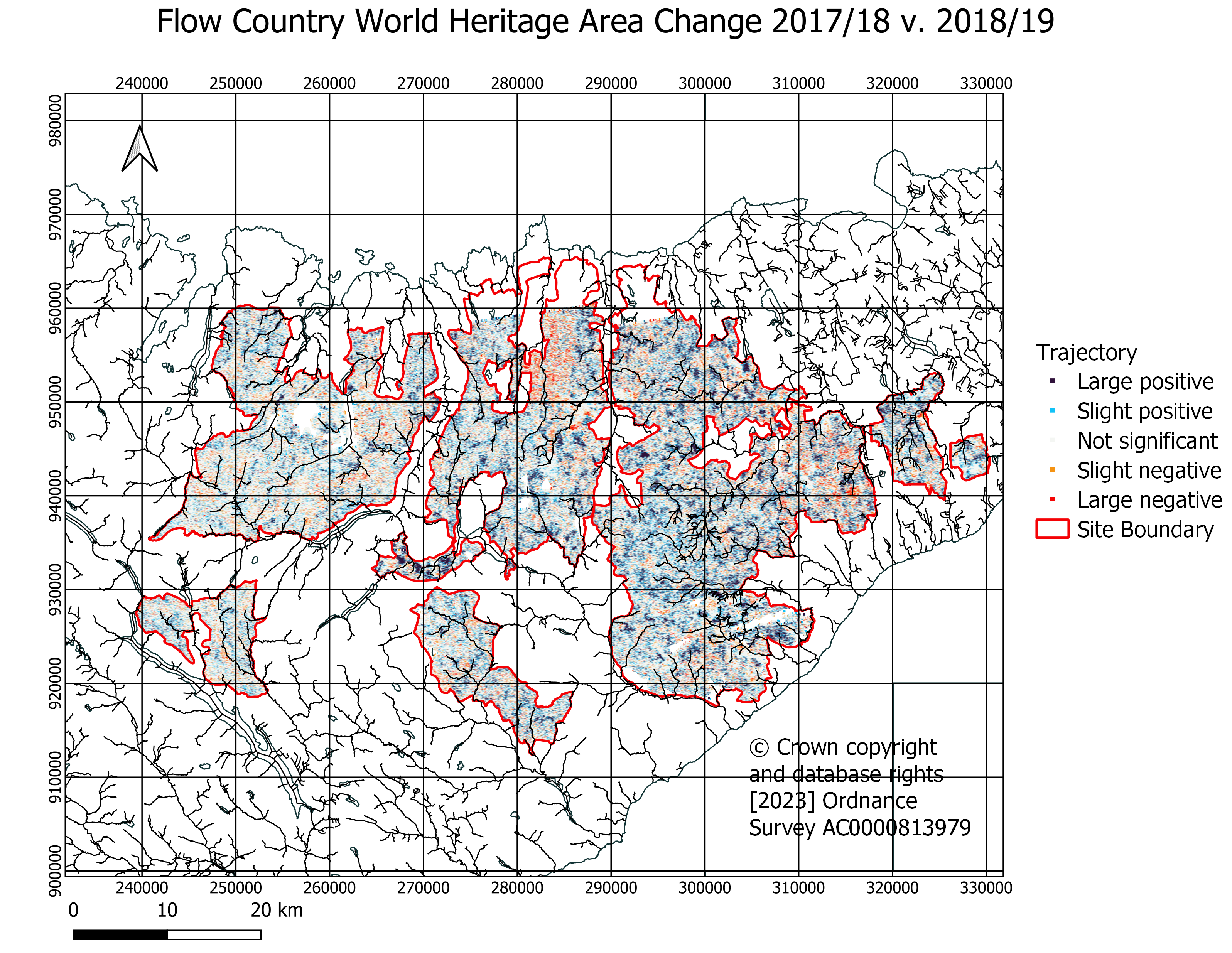
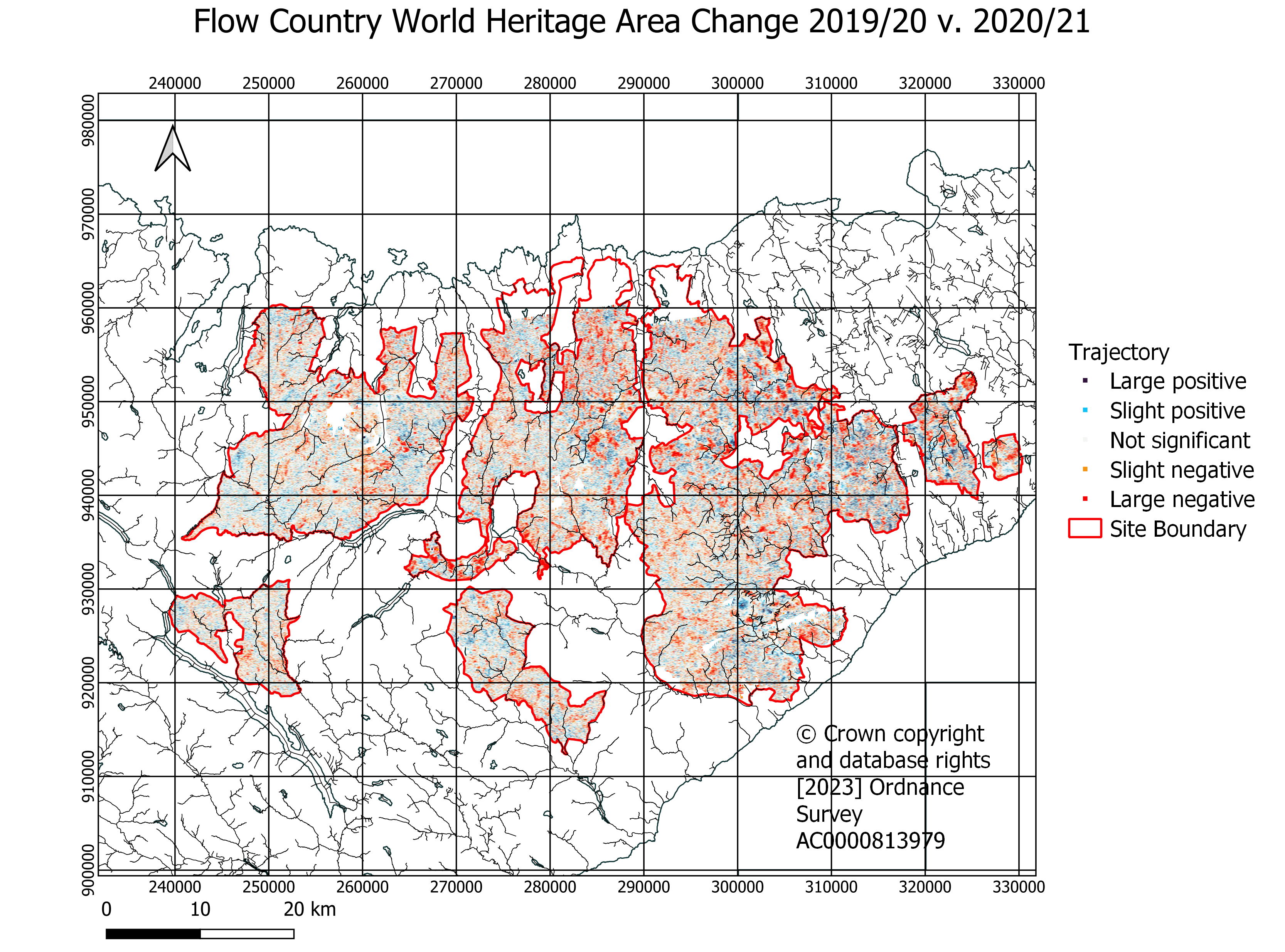
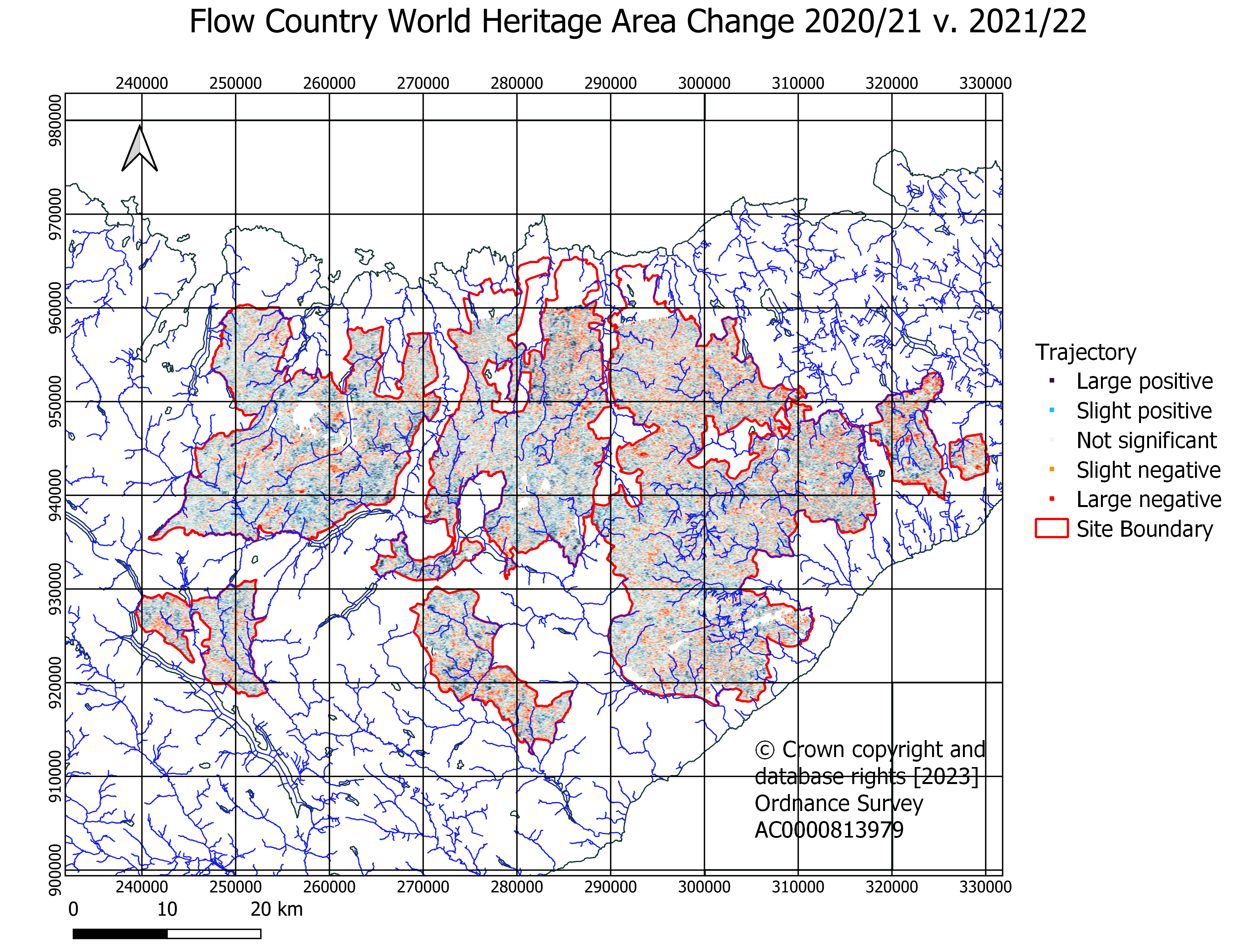