NatureScot Research Report 1410 - Assessment of deer survey methods
Published: 2026
Authors: Fiona M Underwood (FM Underwood), David Recchia (Drone Wild), Charles Hutchinson (Hutchinson Data), and Ben Harrower (BH Wildlife Consultancy, Drone Wild).
Cite as: Underwood, F. M., Recchia, D., Hutchinson, C., and Harrower, B. Assessment of deer survey methods. NatureScot Research Report 1410.
Author contributions
Fiona M Underwood: conceptual and methodological development, data analysis, project leadership & coordination, writing – original draft, review & editing
David Recchia: carbon-costing analysis, methodological development
Charles Hutchinson: GIS analysis, methodological development
Ben Harrower: conceptual and methodological development, project leadership & coordination, team formation, writing – review & editing.
Keywords
Scotland; deer; “drone surveys”; “helicopter surveys”; “dung surveys”; “camera-based surveys”; “deer population assessment”; “deer management”
Background information
Reliable information on deer populations is essential for helping to deliver effective deer management in Scotland, yet no single survey method performs consistently well across all landscapes, species, and management contexts. This report provides an assessment of current deer survey approaches – including helicopter counts, quadcopter drone surveys, dung-based and camera-based methods. It uses a framework that distinguishes between the ecological (state) processes shaping deer populations and the observation process through which surveys detect and measure them. This framework clarifies what different methods measure, where uncertainty and bias arise, and how results should be interpreted across spatial scales and for different population characteristics.
Using representative Scottish landscapes and case studies spanning open upland, semi-natural woodland, upland and lowland commercial woodland, arable, and peri-urban settings, the report examines how survey methods perform under different ecological and operational conditions, compares their operational and carbon implications, and identifies priorities for future development.
Main findings
- No single survey method performs optimally across all ecological contexts, landscapes, and management objectives. Survey outcomes depend on interactions between aspects of the ecological state process, including species ecology, habitat structure, movement, spatial scale, and management, and aspects of the observation process, including survey coverage, detectability, calibration, and survey duration.
- In open upland landscapes, helicopter, foot, and quadcopter drone surveys can provide broad spatial coverage and useful direct counts of deer abundance and demographic structure. Quadcopter drone surveys using thermal imaging generally improve detectability compared with traditional visual aerial counts (counting with the naked eye from a helicopter) while also having substantially lower carbon costs.
- In woodland and heterogeneous landscapes, detectability becomes the dominant constraint. Quadcopter drones perform best where canopy is open or moderately structured but cannot reliably detect deer under dense canopy or thicket.
- Dung-based and camera-based approaches can provide valuable alternatives in woodland landscapes where direct counts are difficult and may better reflect longer-term patterns of deer utilisation or density change. These methods rely on calibration parameters and measure different population quantities from short-duration direct counts.
- Interpretation of survey estimates can depend strongly on deer movement relative to survey scale. Where deer move easily into and out of survey areas, variation in deer numbers caused by movement may be larger than underlying demographic change. In these situations, population totals may reflect short-term site use rather than stable population size, making trends and management effects more difficult to detect reliably.
- Reliable interpretation therefore requires a better understanding of deer movement. This in turn suggests that population assessment is often needed at broader landscape scales that better match the ecological population. Because landscapes often contain a mixture of habitats where no single survey method performs well, development of integrated approaches that combine complementary survey methods within similar survey periods is important.
- At regional and national scales, assessment depends on integrating information collected across multiple landscapes, time periods, and survey methods, while also accounting for gaps in survey coverage and variation in representativeness. This will require improved analytical frameworks, better coordination and accessibility of survey datasets, and more structured monitoring programmes to support extrapolation and consistent assessment through time.
- The highest immediate methodological priority is improving interpretation of deer abundance and site use in woodland and dense canopy environments, including understanding how different survey methods perform and relate to one another where detectability is constrained.
- A major strategic priority is developing integrated monitoring and analytical frameworks that combine multiple survey methods, demographic information, and environmental data across spatial scales. This includes gaining a better understanding of existing survey datasets across Scotland and the barriers to their integration, including accessibility, consistency, and representativeness.
- A key operational development priority is strengthening approaches for surveying large open upland landscapes, including evaluation of lower-carbon aerial platforms, fixed-wing UAV systems, automated image analysis, satellite and aerial imagery and sampling-based survey designs.
Acknowledgements
We thank the following people for their valuable input into this report.
Helen Armstrong (Broomhill Ecology), Mike Daniels (University of the Highlands and Islands), Tiago Marques (Centre for Research into Ecological and Environmental Modelling, School of Mathematics and Statistics, University of St Andrews), Cally Ham (Forest Research), Thomas Logan (University of Leeds and University Centre Bishop Burton), Jackie Potts (Biomathematics and Statistics Scotland), and Tom Turnbull (Association of Deer Management Groups) reviewed an earlier version of the document and provided useful comments.
Cally Ham and Thomas Logan also provided information on vehicle-based distance sampling and camera trapping, respectively, which informed the carbon costing exercise. Kevin Masson (Strathconon Estate) provided information about Strathconon Estate, particularly on the resources required to carry out a foot survey. Cristian Navarro Waggershauser (University of the Highlands and Islands) provided advice on camera trapping and the use of genetic methods. Anton Watson (Forestry and Land Scotland) allowed us access to survey reports and data from several Forestry and Land Scotland sites. Bob Burn (independent statistician) provided feedback on the state–observation framework used to structure the report.
We are also grateful to NatureScot for funding this work and to their staff who contributed their expertise, including Jimmy Irvine on helicopter surveys, Jamie Hammond on helicopter surveys and fixed-wing UAVs, David Shaw on foot counts and Sam Foster and Ivana Curuvija for advice on the carbon costing framework. In particular, Dominic Sargent and Willie Lamont guided the development and delivery of the report.
Abbreviations
AI – Artificial Intelligence
BVLOS – Beyond Visual Line of Sight
CAA – Civil Aviation Authority
CV – Coefficient of Variation
FAR – Faecal Accumulation Rate
FLS – Forestry and Land Scotland
FSC – Faecal Standing Crop
GHG – Greenhouse Gas
GIS – Geographic Information System
ML – Machine Learning
REM – Random Encounter Model
RGB – Red, Green, Blue (imagery)
UAV – Unmanned Aerial Vehicle
VLOS – Visual Line of Sight
VTOL – Vertical take-off and landing
SORA – Specific Operations and Risk Assessment
RGB – Red, Green, Blue
APGB – Aerial Photography Great Britain
Contents
- Keywords
- Background information
- Main findings
- Acknowledgements
- Abbreviations
- 1. Introduction
- 2. Scope and structure of the assessment
- 3. The state process for Scotland’s deer
-
4. Observation process for selected census methods
- 4.1 Introduction
-
4.2 Features of the observation process
- 4.2.1 Idealised case – separating state and observation processes
- 4.2.2 Spatial coverage and representativeness
- 4.2.3 Detection, enumeration and classification
- 4.2.4 Calibration and biological conversion
- 4.2.5 Survey duration, timing, and movement during the survey window
- 4.2.6 Statistical inference and modelling
- 4.2.7 Interpreting survey estimates in dynamic populations
- 4.3 Application of observation framework to different survey methods
- 4.4 Summary
- 5. Empirical comparisons of field surveys
- 6. Comparisons of Resource Requirements
- 7. Synthesis
-
8. Future developments and methodological opportunities
- 8.1 Purpose
- 8.2 Improving detectability, enumeration and classification
- 8.3 Scaling coverage: fixed-wing UAVs and aerial systems
- 8.4 Satellite and existing aerial imagery
- 8.5 Sampling-based survey designs
- 8.6 Genetic and DNA-based developments
- 8.7 Camera approaches to movement and exchange
- 8.8 Integration, modelling and monitoring design
- 8.9 Emerging approaches
- 8.10 Overall perspective
- 9. Design brief priorities for methodological development
1. Introduction
This report is the outcome of a project which aims to help NatureScot determine the most appropriate and reliable methods to support effective evidence-based deer management whilst also ensuring that the methods employed provide value-for-money and have low environmental impact.
Reliable information on deer populations is fundamental to effective deer management in Scotland. Survey data are used to guide culling decisions, assess ecological impacts, monitor long-term population change, and evaluate the success of management interventions. However, obtaining reliable estimates is challenging because deer occur across a wide range of landscapes, at different spatial scales, and under varying ecological and operational conditions.
This project is especially motivated by the rapid technological changes that have led to new tools such as drones, (a term used to describe any unmanned aerial vehicle (UAV)), being used to survey deer across multiple habitats. This method is now reaching a point where it may challenge the use of helicopter surveys which are typically used to assess red deer populations on open hill, but cannot survey the surrounding woodlands. This project provides an opportunity to carry out an evidence-led comparison of the use of helicopters, UAVs and other existing and new technologies to assess deer populations.
The project is built around two stages: first, an independent assessment of the different deer survey methods; and second, a design brief that sets out priority areas and promising directions for further development, including field testing of survey methods, analytical frameworks and monitoring designs to improve deer population assessment.
2. Scope and structure of the assessment
This chapter outlines the scope and structure of the assessment including the objectives, scales, landscapes and survey techniques being reviewed. It defines a framework for assessment and outlines the structure of the report.
2.1 Objectives
The methods this report reviews are designed to estimate the number or density of deer at a site over the length of the survey period. These surveys are typically undertaken for three main purposes:
• To provide a one-off estimate of the number or density of deer within a site
• To measure the impact of a management intervention, such as culling
• To contribute to long-term monitoring of population change
These objectives are closely linked because both the assessment of an intervention and the monitoring of trends depend on reliable estimates of deer numbers at specific points in time. As examples, first, evaluating the impact of a cull requires comparable estimates of abundance both before and after the intervention, ideally compared to changes where the cull did not take place. Second, estimating population trends requires consistent estimates collected repeatedly over multiple survey periods, whether that is to provide relative or absolute estimates.
In many situations, more than just an estimate of the total number, or density, of deer on a site is needed. Estimates may need to be broken down by species, and within species by sex and age class, particularly where data are used to inform population models and guide the setting of culls. In addition, understanding the spatial distribution of deer within a site can be important for interpreting impacts, assessing habitat use, and guiding management actions.
In this report, we begin by assessing how different survey methods perform when used to obtain an estimate of deer numbers or density and their potential to provide disaggregated information, before considering how these same methods can support wider objectives such as evaluating management interventions and detecting population trends.
Throughout this report, estimates are considered for all deer species present in Scotland – red, roe, sika, and fallow deer – recognising that differences in ecology, behaviour, and habitat use influence both the state process and the performance of survey methods.
2.2 Spatial Scales
The spatial scale at which deer population estimates are required varies widely. Estimates may be needed for:
- An individual site, such as an estate or landholding managed by a single owner or organisation
- A larger landscape-scale area, for example one managed collectively by several landowners such as a Deer Management Group
- A regional scale, such as the 11 Wildlife Management Areas, which describe broad regions across Scotland
- The whole of Scotland
In this report, ‘landscape-scale’ refers to analysis at a defined spatial level between site and regional scales. The term ‘landscape’ is also used more generally elsewhere to describe spatial structure and heterogeneity.
At larger spatial scales, it is rarely feasible to survey the entire area at the same time. Instead, estimates of abundance or population trends typically rely on combining information from multiple surveys conducted across space and time. This may involve integrating results from different survey methods or extrapolating from sampled areas to wider regions and is even more challenging the larger the scale (e.g. for a nationwide estimate).
In this report, we begin by considering how survey methods perform at the scale of individual sites, where many surveys are typically designed and implemented, noting that a site can range from a few hectares to a whole Deer Management Group. We then draw these insights together to consider how information from site-level surveys can be combined to inform management, monitoring, and policy at broader landscape, regional, and national spatial scales.
2.3 Landscapes and habitat types
Alongside spatial scale, the ecological setting in which deer populations occur is a central factor shaping how surveys perform and how results should be interpreted. Deer populations in Scotland occupy a wide range of landscapes that present different ecological and practical challenges for population assessment, including variation in visibility, terrain, habitat structure, and deer species and behaviour.
To reflect this, the assessment in this report considers a set of representative scenarios that capture the main ecological and operational conditions under which deer surveys are conducted. These scenarios are: open hill, upland commercial forestry, semi-natural woodland, lowland commercial or mixed woodland, arable, and peri-urban settings. They are used throughout the report to examine how survey methods perform under differing environmental conditions and management contexts, including comparisons of cost, feasibility, and reliability.
In practice, management areas often consist of mosaics of several habitat types rather than a single uniform habitat. Later sections therefore extend the discussion from individual scenarios to more complex mixed landscapes and larger-scale contexts, where multiple survey approaches may need to be combined.
2.4 Survey methods being assessed
NatureScot defined a set of field-based methods to review. These methods were distinguished by: type of technology that is used to cover the ground - helicopter surveys, quadcopter UAV surveys, foot counts, vehicle-based surveys, and fixed cameras; whether deer are recorded directly or inferred from indirect signs such as dung; and whether methods assume that all deer present in surveyed areas are observed, or incorporate approaches to account for animals that are present but not seen e.g. distance sampling.
Many of these methods have multiple variants and protocols, so the review focuses on recognised best practice or the most commonly used approaches. For example, distance sampling (Buckland et al, 2015) can be applied in different ways depending on how the ground is covered. Discussions with NatureScot led to a focus on its use within vehicle-based surveys.
Historically, helicopter and foot surveys have been most frequently applied on open ground in Scotland, while dung surveys, and to some extent vehicle-based surveys, have been more widely used in wooded environments. The first three of these approaches have formed the backbone of deer monitoring in Scotland over the past two decades. In contrast, over the last three to four years quadcopter UAV surveys have increasingly been adopted across a wide range of terrains. In this review we focus on Scotland’s established best-practice UAV methodology (NatureScot, 2026a,b), which uses quadcopters equipped with thermal, optical, and zoom cameras and visits a set of flight points from which the full extent of the site can be surveyed and a minimum count produced. This differs from several UAV approaches described in the literature that either more systematically cover the whole or part of the site using transects and/or do not use thermal imaging and therefore differ in what they observe.
Fixed camera approaches are also beginning to be applied in the UK for large mammals, primarily, though not exclusively, for monitoring feral pigs. NatureScot has recently commissioned work to explore the most appropriate fixed camera methodologies for estimating deer abundance and juvenile survivorship. In this report we focus on the Random Encounter Model (REM; Rowcliffe et al, 2008), which has been widely used across a range of species and settings, whilst recognising that alternative camera-based approaches exist and may be explored in future work.
Finally, we noted, but did not review in detail, several emerging or currently less-used approaches, including fixed-wing UAVs, satellite imagery, DNA-based methods, and acoustic monitoring. These methods are not presently used routinely for deer counting in Scotland but may become more relevant as technology, cost, and regulatory frameworks evolve. They are therefore discussed in a later chapter on future directions and methodological development.
We note that as this review focused on field survey approaches, we did not consider different forms of population modelling, or impact assessment tools such as Habitat Impact Assessments (HIAs).
2.5 Requirements of Estimates: Accuracy and Precision
Deer surveys are designed to estimate the number, density, and spatial distribution of deer within a site. The usefulness of these estimates for management depends on how accurate and precise they are, or need to be, for management purposes. These two properties underpin how survey results should be interpreted and are one component of the methods comparison in this report.
One way to understand accuracy and precision is to look at the estimates of the population total that are obtained from carrying out repeated surveys using the same method on a site where the population total remains constant:
- Accuracy (bias) refers to whether estimates, on average, return the true population total. If a survey method consistently under-counts or over-counts deer, the resulting estimates are biased. This may lead to inappropriate management decisions, for example under-estimating population size and setting insufficient cull levels.
- Precision refers to how much estimates of, for example, the population total might vary between surveys, when the underlying population total does not change. Low precision, also known as high uncertainty, when the population total varies a lot between surveys, reduces confidence in results and makes it difficult to detect trends or evaluate management interventions.
While accuracy and precision describe the quality of survey estimates and impact all three objectives, they do not explain why estimates may be biased or uncertain. To understand the sources of bias and uncertainty, it is necessary to consider how survey observations relate to the underlying ecological system. This is addressed through the state–observation framework described below.
2.6 Core Framework: State Process and Observation Process
The state–observation framework provides a structured way to understand how bias and uncertainty arise in deer survey estimates. It separates the ecological reality of the deer population (the state process) from how surveys detect and measure it (the observation process). This distinction is widely used in wildlife population modelling (e.g. Newman et al 2014).
The State Process
The state process describes the true number and spatial distribution of deer within a site and how these change over time. This underlying population state is typically not directly observed. Key factors shaping the state process include:
- Landscape and habitat structure – vegetation, terrain, and spatial heterogeneity influence which species are present, and how they are distributed and move across a site
- Species behaviour and ecology – including population dynamics, herding and territorial behaviour and food preferences and how these vary with time of year, time of day, and weather – which influence activity, visibility, and spatial use of habitat
- Management actions – such as culling, fencing, or disturbance, which modify abundance and distribution
The Observation Process
The observation process describes how survey methods detect and measure the state process. Surveys capture only part of the true population and may do so imperfectly. Key aspects of this process include:
- Spatial coverage – which parts of the site are surveyed and which are not
- Detection, enumeration and classification – whether deer (or other signs being surveyed) that are present in surveyed areas are observed or missed and once detected if they are correctly counted and classified by species, sex and age
- Conversion or calibration – whether additional modelling is required (e.g. converting dung counts to deer density)
- Timing and duration of survey – whether the survey captures a snapshot of the population or integrates information over time
2.7 Report overview
A review of the scientific and applied literature was undertaken to inform this report. This included published research comparing deer survey approaches, methodological guidance, and operational experience from practitioners. The literature review, together with consultation with technical experts and survey practitioners, underpins the framework and evaluation presented throughout this report.
Chapter 3 examines the state process as it applies to deer populations in Scotland. Six representative scenarios are defined, each illustrated by a case study site, to capture the range of ecological and practical conditions under which deer surveys are conducted. These scenarios provide a consistent basis for comparison throughout the report.
Chapter 4 examines the observation process, describing the key characteristics of the survey methods assessed in this study and evaluating them with respect to the observation process characteristics.
Chapter 5 is an empirical comparison of helicopter and quadcopter drone surveys using data from two study areas. These case studies illustrate how differences in detectability, spatial coverage, and population dynamics influence survey outcomes under real field conditions. It also summarises the literature describing reviews of other comparisons.
A comparative assessment of environmental (specifically carbon) costs and operational resource requirements follows in Chapter 6. This considers carbon emissions, alongside personnel requirements, time, equipment and data demands. A detailed carbon costing for quadcopter surveys is undertaken across all six scenarios (via their representative case study site). For three of these, a fuller comparison is carried out across all other relevant survey methods. These analyses are used to inform comparisons between methods.
Chapter 7 provides a synthesis across spatial scales and management objectives integrating findings from the framework, case studies, costing, and literature. This synthesis highlights where current survey methods are robust, where interpretation remains uncertain, and where key limitations arise – particularly in relation to detectability, woodland environments, open populations, large and heterogeneous landscapes, and integration of multiple data sources.
Chapter 8 considers future and emerging technologies, including developments in hardware, software, statistical approaches, and data integration, and evaluates their potential to address current methodological limitations.
Finally, Chapter 9 sets out a design brief, which identifies priorities for future methodological development including field testing of survey methods, analytical frameworks and monitoring designs.
3. The state process for Scotland’s deer
3.1 Introduction
This chapter describes the state process – the ecological reality that the survey methods attempt to measure – in the context of deer populations across Scotland. Three key factors drive the state process - landscape and habitat structure, species ecology, and management. To explore how these interact we define six representative scenarios capturing different combinations of these three factors. For each scenario a specific site was used for illustration. Table 1 summarises information about these sites with respect to the state process, and detailed site descriptions are in Annex 1.
| Landscape / Site | Dominant species | Main sources of state variability (What causes change?) | What site totals represent (Interpretation) | Short-term variability in totals (How noisy?) | Detectability of trends & management (Can change be detected?) |
|---|---|---|---|---|---|
| Strathconon (Open upland) | Red deer (plus small roe and sika populations) | Seasonal movement and distribution (altitude, red stag vs hind); limited movement across boundaries, approaching a closed system | Totals broadly reflect size of core population, though some movement may occur on margins | Relatively stable; spatial distribution changes seasonally | Good if compared at same time of year |
| Torrachilty (Upland commercial forestry) | Red, roe & sika deer | Movement between site (forest) and surrounding landscape (open hill) driven by season and weather; redistribution following culling; open population | Totals mix both population size and movement, especially for red; clearer when interpreted at a broader spatial/temporal scale | Variable between days and seasons | Good (roe) to poor (red); red clearer at a broader spatial or temporal scale |
| Devilla (Lowland mixed woodland) | Roe deer (plus small sika population) | Daily movement between site (woodland) and surrounding landscape (farmland); seasonal territorial restructuring; immigration linked to culling | Totals broadly reflect the local population size when measured under consistent conditions | Variable within day; relatively stable between days | Good if measured at consistent time of day and season |
| Craigellachie (Semi-natural woodland) | Red, roe & sika deer | Intermittent use by red deer from wider range (open population); roe more stable | Totals reflect site use, especially for red deer; more representative of population size for roe | Highly variable (particularly for red deer) | Poor for red deer; trends clearer only at broader spatial scale |
| Agricultural landscape | Roe deer | Daily movement between cover and feeding areas; seasonal redistribution linked to crops and habitat use; movement to and from surrounding farmland | Totals reflect site use within a wider connected farmland population | Variable within day; seasonally variable | Poor to moderate due to changing site use; clearer at broader scale and consistent time of day and season |
| Easterhouse (Peri-urban landscape) | Roe deer | Local movement between fragmented habitats; limited immigration/emigration along connected corridors following disturbance and mortality | Totals broadly reflect the local population size but influenced by connectivity | Relatively stable | Moderate to good if connectivity understood |
3.2 Landscape Structure and Habitat Context
Across Scotland, deer occupy landscapes that vary widely in vegetation structure, topography, spatial configuration, and human influence. These characteristics determine the distribution of suitable habitat, the availability of forage and cover, and the degree to which landscapes form continuous areas or fragmented mosaics.
Vegetation ranges from open upland systems dominated by heath, grassland, bog, and montane habitats (e.g. Strathconon, Invernesshire) to forested environments including commercial conifer plantations (e.g. Torrachilty, Highland), mixed lowland woodland (e.g. Devilla, Fife), and semi-natural woodland (e.g. Craigellachie, Speyside). Open landscapes typically provide extensive grazing and high visibility, whereas woodland environments provide shelter, structural complexity, and strong spatial heterogeneity. Commercial forestry systems are dynamic, with habitat conditions changing through the growth cycle from open clearfell and new planting to dense thicket and closed canopy.
Landscape configuration varies substantially. Some systems form large, relatively continuous habitat blocks, while others consist of smaller patches embedded within a wider mosaic. For example, upland forestry at Torrachilty is situated within a broader open hill landscape, whereas lowland woodland at Devilla is surrounded by farmland and other woodland sites. Semi-natural woodland at Craigellachie forms part of a wider upland–forestry mosaic rather than an isolated unit.
Topography further shapes habitat structure. Upland landscapes such as Strathconon and Torrachilty span gradients in elevation, slope, and exposure, influencing vegetation and climatic conditions. In contrast, lowland and agricultural landscapes tend to be flatter and more fragmented by a greater variety of land uses.
Agricultural landscapes (e.g. northeast Scotland) are typically open and highly connected, comprising arable land, pasture, hedgerows, and small woodland patches. At the most modified end of the spectrum, peri-urban landscapes (e.g. Easterhouse, Glasgow) combine woodland fragments, greenspace, infrastructure, and built environments. In these settings, habitat is fragmented, connections between suitable areas may be constrained, and human disturbance and physical barriers influence local habitat availability.
Together, vegetation structure, topography, and spatial configuration define the habitat context within which deer populations occur and provide the physical framework that interacts with species ecology and management to shape the state process.
3.3 Species Ecology and Behaviour
Species ecology is a fundamental driver of the state process because differences in movement, seasonality, habitat use and social behaviour determine how deer populations are distributed across space and time. Redistribution, defined here as changes in the spatial distribution of animals caused by movement rather than births or deaths, is a key component of this process. These biological characteristics influence how the distribution of deer changes over time and therefore how stable or variable population numbers appear when assessed at different spatial scales.
Whilst red deer, the largest of the four species, are increasingly found in lowland conditions, they are more typically associated with upland and open hill systems (e.g. Strathconon, Torrachilty and Craigellachie) and occur in large, loosely connected populations structured around herds. Hinds are often hefted, remaining within relatively limited home ranges of a few square kilometres, while stags range more widely and may move over tens of kilometres seasonally. Seasonal redistribution between higher and lower ground is common and strongly influenced by season, weather, and forage availability, with animals moving between exposed and more sheltered areas. Some individuals may remain associated with woodland habitats throughout the year, particularly where cover is available.
As a result of this spatial behaviour, red deer populations tend to be relatively stable when viewed across large landscape units, but may appear more variable at smaller spatial scales where individual sites represent only part of a wider population range. For example, at Strathconon the scale of the landscape encompasses much of the routine movement of the population, whereas at Craigellachie red deer use the site intermittently as part of a broader range. In upland forestry systems such as Torrachilty, most red deer may use forest cover during winter or poor weather but spend much of the time in surrounding open habitats.
Roe deer, the smallest of the four species, are generally territorial and occupy relatively small home ranges, particularly in woodland and mixed landscapes (Devilla, Torrachilty, arable sites, and Easterhouse). Their distribution therefore tends to be spatially stable compared with red deer, although daily movement between woodland cover and adjacent feeding areas such as in Devilla, is common.
In roe deer, seasonal biological processes also influence local population structure. In spring, adult females drive away yearlings from the previous year, leading to short-term redistribution and dispersal. Because roe deer maintain territories and require a minimum area to support forage needs, local density may be constrained by carrying capacity. Although roe populations may appear relatively stable at small spatial scales, movement between neighbouring habitats still occurs, particularly where habitat quality or management pressure varies.
Sika deer (for example at Torrachilty) show movement patterns intermediate between red and roe deer. They are typically associated with woodland and dense cover, often showing relatively localised spatial use and more nocturnal or crepuscular behaviour. Seasonal redistribution is generally less pronounced than in red deer, although movement within forested landscapes can still be substantial. Hybridisation with red deer occurs in many parts of Scotland, and sika continue to expand their range.
Fallow deer (although not present in our example scenarios) occur in more limited parts of Scotland and often form relatively localised populations associated with lowland woodland and agricultural landscapes. They often form social groups and may use open and woodland habitats seasonally.
Where multiple species coexist interactions may influence distribution and behaviour. Competition or avoidance may affect local densities and habitat use whilst interactions with livestock, such as sheep, may also influence spatial patterns in some landscapes.
3.4 Management, Culling, and Immigration
Management is another major driver of the state process. Fencing has long been used to control deer populations and remains an important management tool, particularly to support woodland creation and regeneration sites such as through the Scottish Government’s Forestry Grant Scheme. However, maintaining effective fencing across large landscapes can be difficult and costly. NatureScot guidance (NatureScot website) emphasizes that reducing deer numbers through culling is the preferred long-term approach, and organisations such as Forestry and Land Scotland rely heavily on culling as a tool for managing deer populations with the aim of maintaining deer at densities that allow woodland establishment and habitat recovery. As a result, contemporary management combines these approaches using fencing in targeted situations and culling to regulate population size and reduce impacts on forestry, agriculture, and conservation interests.
Management objectives vary. Conservation-focused estates often seek lower deer densities to protect woodland regeneration and support climate and biodiversity targets. In contrast, sporting estates may maintain higher deer densities to increase stalking opportunities. These differing objectives can create spatial variation in density across neighbouring areas.
Culling affects not only population size but also behaviour and spatial distribution over both short and longer time scales. In the short term, culling can influence short-term behavioural patterns, including shifts in activity timing and habitat use. For example, increased disturbance associated with culling, particularly where night shooting is used, may lead to more nocturnal behaviour or increased use of cover (e.g. Boer-Cueva et al., 2026, Eggers et al., 2026).
Over longer time periods, management actions such as culling can also influence the distribution of deer through movement between areas. Culling in some areas, may lead to immigration from surrounding areas – sometimes described as a vacuum or sink–source effect (e.g. Waber et al., 2013). The magnitude of this effect depends on the intensity of management intervention, species, connectivity, habitat suitability and spatial scale both in the managed and surrounding areas. At large spatial scales, intensive culling may result in a reduction in the population size within the culled area by the number of deer culled (e.g. the regeneration zones at Mar Lodge, Abernethy, or Glenfeshie). At smaller scales, however, immigration from adjacent areas may offset removals. For example, in some forest sites with relatively high densities of roe deer, there may be little or no change in population numbers within the culled area itself, even though there is a reduction in deer numbers at the larger scale. This may be particularly the case when culling is focused in preferred habitats and surrounding areas are subject to lower or no culling.
Cull records provide an independent measure of removals from the population and, when interpreted as an additional observation window alongside survey estimates, can help distinguish true demographic change from redistribution driven by movement.
3.5 Population movement, spatial scale and relationship between survey area and population range
The scenarios described in this chapter relate specifically to the site scale – often the scale at which surveys are requested. However, site boundaries do not always coincide with ecological boundaries (for example red deer at Craigellachie or Torrachilty).
The interpretation of population estimates depends critically on how the survey area relates to deer movement. In population ecology, systems are often described as “closed” when there is no movement into or out of the survey area, and “open” when immigration and emigration occur. These terms are useful because they clarify whether changes in population totals reflect demographic processes alone or both demography and movement.
In practice, fully closed populations are rare in free-ranging deer systems. Movement across boundaries occurs to varying degrees depending on species, landscape structure, season, and spatial scale. Fences are rarely 100% secure. A survey area may also approximate closure over short periods if it contains routine movement of the population – that is, the regular, predictable movements of deer within their normal range (such as daily foraging), but may also behave as an open system for that, or another, species in the same landscape or over a different period of time.
The degree to which a population is open or closed is crucial in understanding what information population totals provide about population size, trend, and management effects.
3.5.1 Closed systems
Of course, no system is ever closed, but we consider here systems that approach closure.
In systems where the survey area contains the routine movement of the population, the total number of deer within a site represents the demographic population size. Redistribution alters spatial distribution within the site, but if no births or deaths occur the total remains unchanged. Population estimates therefore provide a direct measure of population size, and changes over time reflect true demographic change.
In such systems, both population trends and responses to management can be detected reliably. For example, at Strathconon, the large spatial scale encompasses most routine movement of the core red deer population, and so population totals largely reflect demographic processes, including the effects of culling, although some movement across boundaries and seasonal redistribution still occur.
Similar principles apply in systems dominated by territorial species where the survey area exceeds the scale of individual territories. This is illustrated by the woodland roe deer system at Devilla. At the scale of Devilla, the roe deer population total varies within a day due to regular movement between woodland cover and surrounding farmland but is relatively stable between days when measured at consistent times. The population is therefore not fully contained within the survey area, but its spatial structure is persistent and predictable. The main sources of state variability arise from (i) within-day movement between woodland and feeding areas, (ii) seasonal territorial processes, particularly spring restructuring, and (iii) immigration and redistribution associated with management both within Devilla and in the surrounding landscape.
The first process primarily reflects redistribution rather than true population change. In contrast, seasonal restructuring and immigration associated with management can represent genuine demographic change at the site scale, as animals moving into the area may replace those removed through culling or contribute to longer-term population adjustment. Because movement occurs largely within the survey area and follows a stable spatial structure, longer-term trends and responses to management are generally detectable, provided surveys are conducted under comparable conditions.
In both these cases, to accurately assess population trends, or the impact of management interventions, populations should be assessed at comparable points in the annual cycle. This will reduce seasonal variability in deer numbers associated with recruitment and territorial change. In addition, for Devilla, population comparisons should be made at the same time of day to remove the variability caused by daily movement. Under these conditions, changes in population totals more clearly reflect underlying demographic change rather than short-term redistribution. External factors such as severe winters may also influence survival independently of management and should be considered when interpreting change.
3.5.2 Open systems
In contrast, where the survey area represents only part of a wider movement range, movement and redistribution dominate variation in site totals, and population totals may change substantially over short periods. In these systems, site totals primarily reflect the number of animals present at the time of survey, rather than a contained demographic population, and may vary independently of underlying population size.
For example, at Torrachilty and Craigellachie, red deer frequently use these sites as part of a wider range, often in response to weather, forage, or disturbance, and site totals may fluctuate independently of larger scale demographic processes. Immigration into the site does not necessarily represent real population change at the site scale as animals moving into the site may simply be redistributing from other parts of the wider population rather than increasing the overall number of deer associated with the broader system. As a result, short-term changes in site population totals often reflect movement rather than sustained demographic change.
If this variability in the population total caused by redistribution is large, especially relative to the scale of wider population changes, detecting trends or evaluating management at the site scale becomes more difficult. In such situations, interpretation may require broader spatial or temporal context, and measures reflecting longer-term patterns of site utilisation may be more informative than short-term counts.
3.6 Summary
The state process in Scottish deer populations is shaped by the interaction of species ecology, landscape structure, management, and spatial scale. Populations may behave as open or closed depending on context, and population totals may represent population size or site use.
Across all systems, the key determinant of whether population totals provide clear information about size, trend, or management impact is the magnitude of demographic change relative to background variability caused by movement. Where management-induced or natural demographic change is large relative to this variability, for example roe deer, or in red deer at large spatial scales, change can be detected reliably. Where variability is large relative to demographic change, such as red deer at a small spatial scale, interpretation becomes more uncertain and may require broader spatial or temporal context.
Understanding this ecological foundation is essential before evaluating observation methods. The following chapter examines how survey techniques interact with this state process, and how differences in coverage, detectability, and inference influence the accuracy and interpretation of deer population estimates.
4. Observation process for selected census methods
4.1 Introduction
This chapter examines how deer populations are measured in practice, referred to here as the observation process. It focuses on how different survey methods detect, measure, and infer information about deer population size and structure. Chapter 3 described the state process, the ecological reality governing where deer occur, and how populations change, in response to landscape, species ecology and management. Survey methods attempt to measure this ecological state but do so imperfectly and understanding these limitations is essential for interpreting survey results.
Surveys aim to measure populations characteristics such as the population total, the spatial distribution of deer, species composition, and demographic structure (such as sex and age).
Throughout this chapter, the term site is used to refer to the area of interest for which population estimates are required. Surveys may observe all or part of this site, and inference is typically made from the observed areas to the site as a whole.
It is therefore important to distinguish between the population characteristics of interest and what is inferred from a survey. For example, true population total – the actual number of deer present in the site at a given time –can differ from the estimated population total, which is the number inferred from a survey. Differences between these arise from limitations in the observation process.
These limitations arise from several key aspects of a survey that influence how much of the population is captured and how reliably it is measured:
- Spatial coverage – which parts of the site are observed. Some surveys attempt full coverage, while others observe only selected areas, potentially using some form of sampling designs. In practice, even surveys that aim for full spatial coverage rarely achieve this, especially in forested environments.
- Detectability and enumeration/classification – whether animals (or their signs) present in the surveyed area are detected. Conditional on detection, variability may arise in how animals are identified and counted, including classification by species, sex or age, group size estimation and potential double counting. Detectability varies with the state process (e.g. habitat, weather, and deer behaviour and body size), and with survey design and equipment.
- Calibration and conversion – whether the quantity observed (e.g. pellet groups, camera encounters, detected groups) must be converted into an estimate of population size using biological or behavioural parameters.
- Survey time window – the period over which data are collected. Short surveys aim to approximate a snapshot, while longer surveys integrate information over days, weeks, or months, allowing redistribution during the survey period.
In interpreting survey estimates, it is important to distinguish between real changes in the population, and differences in how the population is observed. Ecological change may also occur between surveys through births, deaths, immigration, emigration, or redistribution (Chapter 3) while different survey methods combine the elements of the observation process in different ways.
Variation between survey estimates may therefore arise because the population has changed, because different parts of the population were observed, because detectability differed, or because conversion and time-window effects altered the relationship between observation and true abundance.
4.2 Features of the observation process
Survey methods do not measure deer populations perfectly. Instead, they produce estimates shaped by the observation processes described above, which influence both bias – systematic difference between the estimated and true population total – and precision – the repeatability of estimates under similar conditions.
To understand how these sources of bias and imprecision arise, it is useful to distinguish ecological variation in the state process (Chapter 3) from variation introduced by the observation process. A useful starting point is an idealised situation in which observation error is removed.
4.2.1 Idealised case – separating state and observation processes
Chapter 3 showed that deer numbers and distribution vary through demographic processes and movement across space. To understand how surveys measure these changes, consider an ideal survey that achieves complete spatial coverage of a site and detects and counts every deer present in the survey area in an instant.
In this situation, the estimated population total equals the true population total, and any variation between repeated applications of the survey reflects only ecological change in the state process.
Under this ideal case:
- Changes in estimated population totals between surveys reflect real demographic change or movement into and out of the site between surveys.
- If the true population total remains the same but deer are redistributed across the site differently in repeated applications, the estimated population total remains the same even though the deer locations, and potentially habitat use, may differ.
This ideal provides a reference point. In practice, surveys depart from it through limitations in the observation process that introduce bias and imprecision even when the true population total remains unchanged.
4.2.2 Spatial coverage and representativeness
Surveys differ in how much of a site they cover and how well they represent parts of the site that are not surveyed.
Some surveys are designed as sample surveys (dung, camera, distance), that observe only selected parts of the survey region. Reliable inference of population totals depends on sampled locations representing the site. Systematic or stratified designs are often used to improve representativeness.
If sampled areas are unrepresentative – for example disproportionately sampling areas with high densities and omitting those of low densities, targeting open feeding areas whilst omitting refuge habitats, or sampling from roads where animals might not be distributed at random with respect to the road – estimates may be biased.
Because sample surveys are designed only to survey parts of the site, statistical methodologies exist to estimate the precision of the estimated population total (or other quantity). The precision of these estimates generally increases with the number of sample locations, although some balance between the number of sample locations and the size of each sample area is needed, with more locations improving representativeness and larger sample areas reducing variability within each location. Precision is also higher when deer are distributed evenly across the sampled area so the number of deer within each sampled area is similar (as might happen with roe deer) and will be lower when deer are not distributed evenly across the survey area (as tends to be the case for red deer).
In the context of surveying deer in Scotland, other approaches (helicopter, foot, quadcopter drone) typically aim to cover the entire site. In practice, complete coverage is not generally possible. Areas may be omitted because of vegetation, terrain, access, or survey constraints. Because these are designed to be census counts there is typically no estimate of precision for the estimated population total, since the assumption is that all animals have been seen and counted.
If unsurveyed areas are expected to have similar deer densities to surveyed areas, and both areas are clearly denoted, it may be possible to extrapolate from the surveyed to unsurveyed areas (as with a sample survey), and potentially fit statistical models to get estimates of precision. If, however, as is often the case, unsurveyed areas differ systematically from surveyed areas – for example dense woodland, thicket, or refuge habitat, where population densities are different to those of surveyed areas – extrapolation is not appropriate and the number counted, for a closed population, becomes a minimum count and is biased low.
4.2.3 Detection, enumeration and classification
Even where spatial coverage is complete, not all animals present may be detected. Imperfect detection leads to underestimation of the true population total unless detection probability can be estimated and adjusted for, which is the case for some survey methods – notably distance sampling by construction, and camera traps given additional “work”. The absence of a quantified precision estimate when detection is not perfect does not imply that results are precise; rather that uncertainty in detection remains unmeasured.
Detectability is determined by both the state process and the observation process, reflecting how animals are distributed and behave within the site, and how effectively the survey method allows them to be observed. For example, from the air, large groups of red deer may be more easily detected than individual roe deer, and the use of thermal imagers may detect more individuals than the naked eye.
At its most extreme, animals may not be available to be detected. Here, availability refers to whether animals present can be observed at all using a given survey method. For example, deer in dense tree canopy may not be visible from the air but may still be detectable from the ground or through indirect methods such as dung counts.
When animals are unavailable, the probability of detection is zero. In such cases, these areas should ideally be treated, and noted, as unsurveyed. If these areas differ systematically from the rest of the site this leads back to the issue of representativeness described above and can affect how survey results are interpreted and compared. For example, using a survey method aiming to provide complete spatial coverage of a site containing dense thicket; these areas may technically lie within the survey area but deer within them cannot be detected. In good weather, deer may feed in open areas and be visible, leading to a higher estimated population total. In poor weather, deer may remain unobserved in the denser vegetation. The true population total is unchanged, but the estimated population total differs because animals have redistributed into areas of zero detectability.
Once animals are detected, additional error may arise in how they are counted:
- Group size estimation error – miscounting individuals within detected groups.
- Double counting – counting the same individuals or groups more than once, particularly when animals move during the survey window or when coordination between observers is imperfect.
- Misclassification – not identifying characteristics of the individuals correctly, for example species, age or sex.
These errors influence both bias and precision and are often managed through survey design and field methods, including coordinated survey movement, recording the spatial position of detections that are made, and photographic verification.
4.2.4 Calibration and biological conversion
Some survey methods do not count animals directly but instead measure an indirect quantity that must be converted to abundance, introducing additional uncertainty and potential bias. Examples include:
- converting dung pellet counts to deer density,
- converting camera encounter rates to density,
- converting groups of individuals detected into number of individuals
- any method requiring biological or behavioural parameters such as defecation or movement rates.
If calibration relationships are correct on average, estimates may be unbiased. If calibration is incorrect, estimates may be systematically biased. Even when unbiased, calibration increases uncertainty because biological rates vary across species, seasons, diets, and habitats. However, it is not always the case that the estimate of uncertainty, or variability, in these calibration parameters is propagated into the final precision estimate. This means that the precision of the estimator is overestimated, and inferences made might be incorrect.
4.2.5 Survey duration, timing, and movement during the survey window
Survey methods differ in how long they take to collect data and when observations occur. This affects both what population quantity is measured and how variation should be interpreted.
Short-duration surveys aim to approximate a snapshot of abundance. When surveys extend over multiple days or nights, redistribution during the survey window can alter which animals are observed, adding variation even when total abundance is unchanged.
Long-duration surveys integrate information over weeks or longer and may reflect average abundance or site use rather than instantaneous abundance. Changes in population size or distribution during the survey period can influence interpretation, so particular care is needed for open populations
4.2.6 Statistical inference and modelling
In addition to the core components outlined above, some survey methods use statistical models to infer population size or density from partial observation. Examples include modelling detection probability, extrapolating density from sampled to unsampled areas, or estimating density from encounter rates.
These models formalise assumptions about detectability, spatial representativeness, and population behaviour, and allow uncertainty to be quantified. However, estimates are only as reliable as the assumptions on which the models are based. Violations of these assumptions may introduce bias.
4.2.7 Interpreting survey estimates in dynamic populations
These components and modelling approaches together determine how survey results should be interpreted. Variation in survey estimates may arise from the observation process rather than real changes in the state process When this observation-related variation is small relative to real population change, surveys can reliably detect trends and management effects. Where observation variability is large relative to underlying change, detecting real change becomes difficult. This relationship determines the effective power of monitoring and influences how survey results should be interpreted.
4.3 Application of observation framework to different survey methods
4.3.1 Introduction
The observation framework described above is applied here to each of the main survey methods considered in this report. These methods differ in how they achieve spatial coverage, how detectability and availability are addressed, whether calibration is required, and how the survey time window influences interpretation.
Table 2 summarises these key components across methods and provides a basis for comparing their outputs and understanding their strengths and limitations. This table, in general, assumes that method assumptions hold (according to best practice and published methods) and some sources of bias and precision may occur if this is not the case.
| Method | Primary output | Survey coverage | Detectability | Calibration required | Time window / population quantity measured | Precision / uncertainty quantified? | Main sources of bias | Typical habitat / best use |
|---|---|---|---|---|---|---|---|---|
| Helicopter surveys | Number of red deer, sex and age, observed during survey period and spatial distribution; usually interpreted as a minimum count over large areas | Near-complete in open landscapes; partial where poor detection | Generally high in open terrain but reduced by vegetation, terrain, and conditions; detection not modelled; | None (direct count) | Snapshot of abundance over survey window (usually 1–2 days) | Influenced by coverage and detectability; rarely formally quantified (no explicit detection or sampling variance estimated) | Missed animals in cover; incomplete coverage; redistribution into low-visibility habitats; movement during survey | Large open upland landscapes; rapid large-scale counts |
| Quadcopter drone (thermal) surveys | Number, species, sex, age and spatial distribution of deer observed; usually interpreted as a minimum count unless coverage complete | Designed for near-complete coverage but gaps may remain due to poor detection, access, or weather | Depends on thermal contrast; reduced under dense canopy, thick vegetation, or warm conditions; detection not usually modelled | None for direct counts | Approximate snapshot of abundance over survey window (single session to several days) | Influenced by coverage and detectability; usually not formally quantified unless extrapolation or modelling applied | Unsurveyed areas; missed animals in dense vegetation or low thermal contrast; redistribution into canopy cover; movement during survey | Open terrain and moderately structured woodland; spatial mapping; high-resolution surveys |
| Foot (ground) counts | Number of (red) deer, sex and age observed at time of survey; typically a minimum count with species and demographic information where possible | Often near-complete in open terrain; partial in wooded or complex landscapes | Visibility-dependent; reduced in vegetation or complex terrain; detection not modelled; group counting and double counting may occur | None (direct count) | Snapshot of abundance at time of survey (single session to several days) | Influenced by coverage and detectability; usually not formally quantified | Incomplete coverage; missed animals; double counting; redistribution during count | Open hill landscapes; coordinated counts over defined areas |
| Vehicle distance sampling | Estimated deer density over survey period, usually with confidence intervals, and potentially by species, age, sex | Sample survey along transects; depends on representativeness of transects relative to landscape | Detection explicitly modelled as a function of distance; assumes perfect detection on transect; influenced by vegetation, terrain, weather; group size estimation required | Conversion from group density to individuals using mean group size | Average density over survey period (assumes short-term closure), (several nights) | Formally quantified through sampling and detection modelling | Unrepresentative transects; violation of detection assumptions; incorrect group size; unmodelled detectability variation | Woodland with track access; moderate visibility |
| Dung (pellet group) surveys | Estimated deer density or site use over accumulation period with uncertainty | Sampled plots or transects; depends on representativeness and coverage of habitats | Detection relates to finding pellets, usually assumed to be high; affected by vegetation, substrate, and observer performance; sometimes modelled | Conversion from pellets to deer requires defecation rate and pellet persistence (derived from decay processes), parameter uncertainty can be incorporated | Accumulated site use over survey period (weeks to months) | Formally quantified if sampling and all calibration uncertainty included | Mis-specified defecation rate or pellet persistence; non-representative plots; pellet misidentification; population change during survey window | Woodland; useful where direct observation difficult; longer-term density or utilisation |
| Camera trapping (Random Encounter Model) | Estimated deer density over deployment period with uncertainty, often species-level | Sample of deer activity at camera locations; depends on representative placement | Detection occurs when animals pass camera detection zone; influenced by vegetation, placement, and behaviour; explicitly modelled | Requires calibration of moving and camera detection zone geometry | Average density over deployment period (weeks to months) | Formally quantified through modelling of sampling and calibration uncertainty | Unrepresentative camera placement; incorrect movement or detection parameters; violation of independence or closure assumptions | Wide range of habitats; long-term density or utilisation where direct observation difficult |
4.3.2 Helicopter surveys
Helicopter surveys are a long-established aerial count method used primarily to estimate deer numbers across large open landscapes, particularly upland red deer systems in Scotland. NatureScot has used helicopters for their red deer counts since 2001 and has published best practice on their use (NatureScot 2008a,b).
One or more helicopters systematically cover the target survey area while trained observers detect deer visually from the air. Large groups are frequently photographed to support later verification and to minimise counting error. For each observation, the location, group size, and where possible sex and age composition are recorded. The primary output is the location of groups of deer observed within the surveyed area during the survey period, typically broken down by sex and age, leading to a total (minimum count) estimate over the whole region.
NatureScot publishes these data (NatureScot 2025), and summaries at the scale of 10km squares. However, because clearly defined survey boundaries are not provided it can be difficult to identify the exact area surveyed, limiting the wider use of these data, including modelling changes over time, and comparison or integration with other datasets.
Survey coverage depends on the ability to visually search the landscape from the air. In extensive open habitats with relatively continuous terrain, helicopter surveys can approach near-complete coverage over large spatial scales. In these conditions, detectability is generally expected to be high, especially in winter when vegetation cover is low and deer may be highly visible against snow. Detectability can decline where ground vegetation (e.g. bracken, heather, rhododendron), broken snow cover, or poor light conditions obscure animals.
In more complex landscapes, particularly those containing woodland, dense vegetation, or fragmented terrain, some areas may remain unsurveyed. In practice, areas of dense conifer are often excluded from surveys, as deer within them are not visible from the air, and flight paths may be designed to avoid these areas.
Behavioural response to the helicopter can sometimes improve visibility, although deer do not respond consistently. In less dense woodland, helicopters, or in some cases additional people on the ground, may be used to move deer from woodland into adjacent open ground to improve coverage, although this is not always effective as deer may be reluctant to break cover and so turn back into the wood.
Counting error, group size estimation, and duplication of moving groups can affect accuracy, and survey design aims to minimise these through flight planning and photographic verification of observed numbers of deer.
Helicopter surveys are often described as snapshot counts, but in large areas they may extend over more than one day. During this period, deer movement and redistribution between habitats can alter the spatial distribution of animals and contribute to variation between surveys even when total abundance is unchanged. Careful survey planning can minimize this effect.
Bias may arise if areas are incompletely covered, if animals remain undetected in vegetation or woodland, or if movement during the survey leads to under- or over-counting. Because detection probability is not explicitly estimated, missed animals cannot be accounted for formally so final estimates are a minimum count with no formal quantification of uncertainty.
Helicopter surveys are most effective in large, open landscapes where visibility is high and continuous coverage can be achieved, and are less reliable in forested, densely vegetated, or highly fragmented habitats where detectability and coverage are reduced.
4.3.3 Quadcopter (UAV) surveys
Quadcopter drone surveys aim to count deer across a defined area using airborne thermal imaging. This methodology has become more common over the last five years. Here we assume Best Practice guidelines (NatureScot 2026a,b) are adhered to. Quadcopter drones are typically flown from a series of pre-planned launch points arranged to provide complete spatial coverage of the site. From each position, the drone surveys the surrounding landscape using a thermal camera to detect individual animals, while RGB (red, green, blue) zoom imagery is used to confirm species and group characteristics. The primary output is location of deer groups within the survey area as well as where possible, their species, age and sex. This is combined with spatial information on the boundaries of surveyed and unsurveyed areas to provide a minimum count and minimum density estimate.
Although designed to approximate a complete count, full coverage of the site and perfect detectability is not always achievable. Areas may remain unsurveyed due to a variety of constraints including access, line-of-sight limitations, weather, or dense vegetation such as closed canopy forest or thicket where detectability is poor. Survey protocols require that unsurveyed areas are recorded, together with reasons for their exclusion. Where unsurveyed areas are small, structurally similar to surveyed areas, and deer density could be assumed to be similar to surveyed areas, extrapolation may be possible, though it introduces uncertainty. Where omitted areas differ substantially, extrapolation is not employed, so results should be interpreted as a minimum count.
Detectability in quadcopter drone surveys depends primarily on thermal contrast between animals and their surroundings and is influenced by vegetation structure, weather, and time of day. Detection is typically high in open habitats, non-leafed woodland, and cool conditions, but declines under dense canopy, thick understorey, or sunny conditions when thermal contrast is reduced. As for helicopters, detection probability is not normally estimated explicitly, so undetected animals cannot be corrected for formally.
Counting error, species misclassification, and duplication of moving animals can affect accuracy. Communication on the ground and post-processing of imagery is used to minimise these risks.
Drone surveys may be completed within a single session or over multiple days in larger areas. Redistribution can alter spatial distribution and influence the proportion of the population observed, so careful planning is required to minimize this risk.
Bias may arise if areas are incompletely covered, if animals remain undetected in dense vegetation or low-contrast conditions, or if movement during the survey leads to under- or over-counting. The level of precision is dependent largely on detection issues and cannot be formally quantified, because detection probability is not explicitly estimated.
Quadcopter drone surveys are particularly effective in open landscapes and moderately structured woodland but are more limited in dense forestry, commercial conifer or seasonal cover from deciduous trees, where both coverage and detectability constraints are greatest.
Other UAV-based survey methods exist including sampling the survey area or covering the area systematically using transects.
4.3.4 Foot counts
Foot (ground) surveys are direct counts in which teams of observers walk predetermined routes or occupy coordinated vantage points to count deer across a defined area. The method is widely used in open hill landscapes, especially for red deer and NatureScot has published best practice guidelines for these (NatureScot, 2008a,b). Observers record the location, group size, and characteristics of deer observed. In some surveys, thermal imagers may be used to assist detection, particularly under low-light conditions or where visibility is reduced. Larger groups are often photographed to support later verification. The primary output is the number of deer observed within the survey area at the time of survey, typically broken down by species and, where possible, sex and age, and generally representing a minimum count unless full coverage and high detectability are assumed.
The surveyed area may approach full coverage in small or moderately sized open landscapes where observers can maintain coordinated lines of sight. In larger, more complex, or wooded areas, some ground may remain unsurveyed due to terrain, vegetation, access limitations, or communication constraints, and counts may therefore represent a minimum number present. Results depend on effective coordination and on observers collectively covering the defined area without gaps or overlap.
Detectability is strongly influenced by visibility, vegetation structure, weather, and deer behaviour. Detection is generally highest in open habitats, particularly under conditions that improve contrast such as full snow cover. Detectability declines where deer remain in woodland, sheltered terrain, or dense vegetation, or where weather reduces visibility. Detectabilty may be lower on flat ground where only deer on the skyline can be observed. Survey design may attempt to increase detection by coordinating observer movement or positioning observers relative to wind and terrain, although detection probability is not explicitly estimated.
Errors in group size estimation, misclassification of sex or age, or duplication of moving groups can affect accuracy. Survey design seeks to minimise double counting through coordination and communication, although effectiveness depends on terrain and species behaviour.
Foot surveys do not require calibration from indirect signs or movement rates, as deer are counted directly.
Counts are usually completed over a few days and aim to represent abundance at the time of survey rather than an average over an extended period, although in some cases the survey may take several weeks due to issues of finding surveyors.
Bias in estimates may arise if areas are incompletely covered, if deer remain undetected due to vegetation or complex terrain, or if movement during the count leads to under- or over-counting. Precision is affected by detectability but because detection is not estimated, uncertainty is typically not formally quantified.
Foot surveys are most effective in open landscapes with good visibility and coordinated access across large areas and are less reliable in wooded or highly fragmented habitats where detectability and coverage are reduced.
4.3.5 Vehicle-based surveys using distance sampling
Vehicle-based surveys estimate deer density from observations collected by driving slowly along predetermined transects, usually forest tracks. Observers use thermal imagers to detect animals from the vehicle, then record species, group size. When using a distance sampling methodology, the distance and angle from the transect to the detection are also recorded. Distance sampling (Buckland et al 2015) uses these distances to estimate detectability and correct the observed number of animals/groups for those missed. This is achieved by modelling a detection function, which describes how the probability of detecting a group of deer declines with increasing perpendicular distance from the transect. This function can incorporate additional information, such as group size and habitat. Together with the observations, this provides an estimate of the density of groups of deer within the survey region which is converted to an estimate of the density of individual deer using a conversion factor, or multiplier, of the average number of deer per group.
The primary output is an estimate of deer density within the surveyed area over the survey period, typically reported with associated uncertainty, and often broken down by species and sometimes group characteristics. Spatial modelling to describe the distribution across the site is also possible.
The surveyed area represents a sample of the whole site; only areas visible from transects are observed directly. Results therefore depend on the transects being representative of habitat conditions and deer distribution across the whole site. In woodland systems where transects are tracks, this assumption may be more reasonable during night surveys when deer are more mobile and less strongly associated with specific habitat features. If transects do not adequately represent habitat conditions – for example where dense vegetation or inaccessible terrain differs in deer density – estimates may be biased.
Detectability should be highest (and perfect on the transect itself) close to the transect line and decline with distance, which is explicitly modelled through the detection function described above. In practice, detectability can also be affected by other factors that limit visibility or thermal performance, such as dense vegetation, complex terrain, weather and moon phase. If dense vegetation increases with distance from the track, conventional distance sampling may not be able to disentangle changes in density with detection (Marques et al 2013). Model selection and measurement error in distance and angle estimation also contribute to uncertainty in the detection function.
Deer density is first estimated for groups and then converted to individuals using mean group size. This adds additional uncertainty particularly when group sizes vary markedly, for example for red or fallow deer, and could be a source of bias if group size is not correctly estimated.
Vehicle-based surveys are often conducted over multiple nights, and the resulting estimate represents average density over the survey period rather than abundance at a single moment. This assumes no substantial population change during the survey window. Careful survey planning can reduce double counting on an individual night by ensuring transects are spaced carefully. Animal movement between nights, provided it occurs at random with respect to the way the survey is being implemented, does not lead to bias.
Precision of distance sampling estimates depends on the precision of the random components in the estimators: the number of individuals seen, variability in the detection function estimation and variability in mean group size. Distance sampling methods allows all of these to be quantified and propagated to the final density estimates.
Bias may arise if key detection assumptions (such as perfect detection on the line) are violated, if group size is incorrectly estimated or if deer density by transects along roads is unrepresentative of the wider landscape.
The method has been repeated annually for over a decade in the Forest of Dean with observers using the same transects each year to track trends over time. It is one of the few methods currently used to survey deer that quantifies uncertainty from multiple sources.
4.3.6 Dung surveys
Dung (pellet group) surveys estimate deer density or utilisation from counts of pellet groups in sampled plots or transects. Rather than counting deer directly, the observed quantity – pellet group density – must be converted to deer density using biological parameters. The number of pellets observed reflects production over a period of time determined by defecation rate and the duration for which pellets remain in the landscape. This duration may be estimated from pellet persistence (derived from decay processes) or defined directly by measuring pellet accumulation over a known interval (see Swanson et al 2008 for a review of different methods). Surveys may include multiple visits to help estimate pellet persistence or accumulation. Because dung accumulates over time, the primary output results typically represent average site use or pressure rather than instantaneous abundance, with a measure of uncertainty and information on spatial distribution of utilisation across the site. Red deer densities may be defined separately from other deer species.
Dung surveys sample only part of the landscape, so representativeness of plots or transects is critical. Survey designs typically distribute plots systematically or randomly across the survey area, sometimes stratified by habitat. Deviating from sampling protocols or preferentially searching high-use areas, such as deer paths, or clustering plots in accessible areas will introduce bias. Some micro habitats may be excluded where pellets cannot be reliably detected (deep litter, dense vegetation, waterlogged ground) which should be recognized when interpreting results.
Here, detectability relates to finding pellet groups rather than animals and is influenced by vegetation, ground cover, observer performance, and pellet condition. Research has indicated that the use of short narrow transects leads to high detectability (Campbell et al 2004). Dense vegetation or heavy litter may reduce detectability and make some habitats effectively unavailable for survey. Some approaches record distance from the centre of the transect to the dung and use distance sampling approaches to account for varying detection.
Once detected, pellet groups must be correctly classified to species. Pellet morphology typically allows reliable discrimination at most between red deer and other deer species. Field identification may also be complicated where non-deer species, particularly rabbits and sheep, are present, as their pellets can be confused with those of deer especially when dung is partially decomposed or sodden by rain-saturated ground. Estimates can therefore be biased if it is not possible to differentiate between deer and other species, especially in areas of high sheep densities, unless corrective adjustments are applied.
Estimating deer density requires calibration, or multipliers, to convert pellet counts to deer numbers. The first multiplier is defecation rate which varies with species, diet, and season. Typically, a standard rate from the literature is applied, not always with an estimate of how this might vary. Without including this variability, the total uncertainty of the estimate is underestimated (and bias can be introduced too).
The second multiplier accounts for the time period over which pellets contribute to direct counts either through estimates of pellet persistence (the average time pellets remain detectable, derived from decay processes) or direct measurements of accumulation. Different survey approaches estimate either pellet persistence or accumulation which vary with weather, habitat, and substrate and diet:
- Faecal Standing Crop (FSC): a single visit approach in which pellet groups are counted and converted to density using an external estimate of pellet persistence in addition to defecation rate. This is sensitive to seasonal and habitat variation in pellet decomposition
- Faecal Accumulation Rate (FAR) / clearance counts: A two-visit approach in which pellet groups are counted and cleared at Visit 1, and new pellet groups counted at Visit 2. This measures accumulation over a known period and removes the need to estimate mean persistence time, assuming pellets do not appear and fully decompose between visits.
- Combination approach (Swanson et al 2008): A two-visit approach that integrates accumulation counts with direct estimation of pellet persistence based on observed decay between visits. On the first visit pellets are marked and on the second the plots are revisited and the number of new pellets as well as the number remaining from the first survey are recorded. This direct estimation of pellet persistence improves calibration where decay varies substantially among habitats or seasons and allows uncertainty in persistence to be quantified rather than assumed.
- In more recent FLS reports, a hybrid design is used in which a subset of transects (e.g. a quarter) follow the FAR approach with two visits, whilst the remaining are surveyed during the second visit using the FSC approach. This improves efficiency whilst retaining information on accumulation rates.
Because surveys typically extend over several weeks, results reflect average site use over the survey period. Changes in population size or distribution during this interval can affect interpretation. Methods that account for “ghost groups” (that is pellet groups produced by deer that have since been culled), using data on deer culls during the survey period, are used to account for some of this potential bias although it does not account for natural mortality during the survey period.
Uncertainty arises from sampling variability and from variation in biological parameters (defecation rate and pellet persistence) across species, habitats, and seasons. Bias arises from unrepresentative survey coverage, misclassification of pellets, unaccounted population change due to ghost groups and incorrect assumptions about the multipliers.
Dung surveys have been used in both woodland, historically across much of the FLS estate, and open upland landscapes across Scotland. Differences from direct counts largely reflect their longer temporal window and reliance on calibration. As with distance sampling it is one of the few methods where all sources of uncertainty are quantified. Dung surveys do not directly provide information on species (beyond red vs other species) sex or age information.
4.3.7 Camera trapping (e.g. Random Encounter Model)
Camera trapping is a passive method in which cameras record photographic or video evidence of deer at fixed locations over extended periods. Cameras are typically deployed in a random or systematic design, so detections represent a spatial sample of deer activity. Images provide time-stamped records of presence, group size, and often species identity, with sex or age sometimes identifiable. The primary output is an estimate of deer density within the surveyed area over the camera deployment period, derived from photographic encounter rates and reported with associated uncertainty, often with supporting information on species and relative activity across the site.
The surveyed area is only a sample of the wider site, and results depend on cameras being placed in locations representative of deer activity across the landscape. Biased placement, for example along high-use trails, feeding areas, or accessible locations, can overestimate density or site use. Some habitats may be effectively unsampled where cameras cannot be deployed, for example dense thicket.
Cameras may be motion-sensored so detection only occurs when animals pass through the effective detection zone of the camera and trigger the sensor. Variation in vegetation, terrain, camera orientation, or sensor performance can influence detection and contribute to uncertainty. Sparse detections, particularly at low densities or with widely spaced cameras, can reduce precision. Alternatively, cameras may record an image every few minutes and detection then depends on the processing of images to identify individuals.
For unmarked deer populations, density is commonly estimated using the Random Encounter Model (REM) (Rowcliffe et al 2008). This approach uses motion-sensored cameras and infers density from the rate of independent photographic detections, camera operating time, the geometry of the camera detection zone, and an independent estimate of animal movement rate. Calibration therefore depends on accurate estimation of detection zone parameters and movement behaviour. Bias may arise if these are mis-specified or vary across habitats, seasons or species.
Because cameras operate continuously, REM estimates represent average density over the deployment period rather than instantaneous abundance. Redistribution, births, deaths, and movement during this period influence interpretation, and assumptions about population closure and independence of detections must be considered.
Precision reflects sampling variability, detection uncertainty, and calibration of movement and detection-zone parameters, all of which can be quantified within the modelling framework. Bias may arise if camera placement is unrepresentative, if detection parameters or movement rates are mis-estimated, or if assumptions of independence and closure are violated.
Camera trapping can be applied across a wide range of habitats with minimal disturbance once cameras are installed. It is particularly useful where direct observation is difficult or where long-term monitoring of population change or site use is required, although performance may decline in very dense vegetation or where detection zones are heavily obstructed.
There is currently a lot of research in the development of camera trapping methodologies for unmarked populations (for a review see Gilbert et al 2021). But there has been very limited use of this method in the UK for deer. NatureScot is investigating how camera traps can be applied to deer within Scotland, including the use of continuous time monitoring.
4.4 Summary
Across all methods, survey estimates are influenced simultaneously by multiple sources of uncertainty, including spatial coverage, detectability and enumeration error, calibration of biological parameters, statistical model assumptions, and movement during the survey window. These components operate together rather than independently. For example, incomplete coverage may interact with deer densities and movement; detectability may vary with weather and habitat; and calibration parameters may vary seasonally.
Some methods, particularly those based on distance sampling or formal modelling frameworks such as REM or calibrated dung surveys, explicitly estimate uncertainty arising from sampling and detection processes. Other approaches, especially minimum-count aerial and ground surveys, do not formally quantify detection probability or sampling variance. Unless the rare conditions for a total count apply, the absence of a reported confidence interval does not imply high precision; rather, uncertainty remains unmeasured. In these cases, results are presented as a minimum count indicating that the number seen is that observed during the survey period where spatial coverage was possible. It is important to retain additional information about surveys to understand how comparable they are, especially when comparing over time.
The ability to detect real population change depends on the relationship between ecological variability in the state process and variability introduced by the observation process. When true population change is large relative to observation variability, trends and management effects can be detected reliably. When observation variability is large relative to ecological change, detecting real change becomes difficult, regardless of whether abundance is estimated from a sample survey or is a complete count. This relationship determines the effective power of monitoring programmes and underpins interpretation of survey results over time.
Table 2 summarises the key information about each survey method. This table, in general, assumes that method assumptions hold (according to best practice and published methods) and some sources of bias and precision may occur if this is not the case.
5. Empirical comparisons of field surveys
5.1 Introduction
This chapter presents empirical comparisons between survey methods using field data. Earlier chapters developed the conceptual framework linking the state process (ecological reality) and the observation process (how surveys detect and measure deer). Here, this framework is applied to real survey data to examine how these processes influence differences between survey estimates.
Two case studies are used. The first (North Arran) represents a largely open and relatively closed system, providing a clearer basis for comparison between methods. The second (Glen Creran–Duror) represents a more heterogeneous and open landscape, where movement, habitat structure, and incomplete spatial overlap complicate interpretation.
The following section describes how comparable survey areas were identified, before the case studies are examined in detail. This is followed by a brief summary of other comparative studies in the literature.
5.2 Identifying overlapping survey sites
To identify comparable survey areas, BH Wildlife Consultancy quadcopter drone survey data were spatially overlaid with NatureScot helicopter survey data and Forestry and Land Scotland (FLS) dung survey data. Drone and dung survey site boundaries conducted since 2021 were mapped directly. Helicopter survey coverage was reconstructed by applying a 500m buffer either side of the recorded flight paths. The coverage should be considered an approximation of the true survey footprint rather than an exact boundary.
Sites under public ownership (e.g. NatureScot or FLS) were identified and screened for temporal overlap between surveys. Two sites were selected for detailed drone–helicopter comparison where survey dates were sufficiently close to minimise ecological change between surveys.
A drone–dung comparison was not pursued because surveys were conducted in different seasons and years, so were not directly comparable. A robust comparison would require surveys in the same season and is recommended as future work.
Two case studies are therefore examined:
- North Arran – helicopter and quadcopter drone survey in a largely open hill closed population system (September 2024)
- Duror–Glen Creran complex – helicopter and quadcopter drone survey in a heterogeneous woodland–open mosaic (March 2024)
Interpretation is based on discussions with the surveyors (BH Wildlife Consultancy for the quadcopter drone survey and NatureScot staff members for the helicopter survey).
5.3 Interpreting differences between surveys
Comparisons between survey methods were interpreted by evaluating alternative hypotheses for the observed differences in population estimates between counts. The aim was to assess whether differences arose from true differences in the underlying deer population (state process) or are due to differences in the survey methods (observation process).
The framework developed in earlier chapters was used to guide this comparison, focusing on relevant components of the state and observation processes. Only those elements applicable to these surveys were considered. For example, both methods aim to directly count animals, so calibration (e.g. conversion from dung to deer) is not relevant here, and survey duration was not considered in detail.
Differences between surveys were examined against the following hypotheses:
Hypothesis 1: Differences arise due to changes in abundance (state process)
Differences between survey estimates may reflect real changes in the number of deer present within the survey area, whether due to mortality (culling in particular) or when populations are open and deer move into or out of the area.
Hypothesis 2: Differences arise due to incomplete or differing spatial coverage (observation process)
Not all areas within the site may have been surveyed. Deer may be in unsurveyed areas during one survey but within the surveyed area during another, meaning that animals may be included in one count but not the other.
Hypothesis 3: Differences arise due to variation in detectability (observation process)
Survey methods may not be equally effective at detecting all deer within surveyed areas, so some individuals or parts of the population are more likely to be detected than others.
Hypothesis 4: Differences arise due to enumeration effects (observation process)
Differences may arise from how animals are recorded, including grouping effects or potential double counting.
5.4 Case Study 1 – North Arran
North Arran (Figure 1) provides a relatively simple system in which to compare survey methods.
5.4.1 State-process context
North Arran, with sea to the north, east and west, is predominantly open hill with patches of broadleaved and conifer woodland and is dominated by red deer. At the spatial scale surveyed, the population behaves approximately as closed over short time periods, with minimal immigration from southern Arran and little culling during the interval between surveys. This provides a relatively stable ecological setting in which differences between surveys are more likely to reflect observation-process effects rather than true population change.
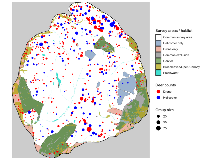
Figure 1. Map of North Arran survey site showing survey coverage, habitat type, and deer observations.
Click for a full description
Points mark the location of deer groups recorded by quadcopter drone (red) and helicopter (blue), using a point scale of 25, 50 and 75 indicating the size of the group. Woodland habitat was classified using the National Forest Inventory as broadleaved/open canopy (yellow) or conifer woodland (green). Areas surveyed only by drone are shown in red, and areas surveyed only by helicopter are shown in blue. Helicopter-only areas occurred because foggy conditions prevented effective drone survey. Dense canopy areas, largely conifer woodland, were generally not surveyed by either method and were excluded from the final comparison. Although some deer were observed by the drone within parts of the conifer woodland, these areas were not surveyed consistently and are therefore classified as exclusions. Final population estimates are compared for the common surveyed area (white).
5.4.2 Observation-process context
The helicopter survey was conducted on 30 August 2024 using one helicopter. The quadcopter drone survey was conducted on 8–9 September 2024 with four operators each day. The drone survey was commissioned specifically to compare with the helicopter survey, and survey design aimed to match helicopter-observed areas as closely as possible. Conifer woodland was excluded from both surveys as neither approach would be able to detect deer. In each case best practice guidelines were followed, and results represent minimum counts of population totals.
5.4.3 Results and Direct Comparison
Across the full North Arran complex excluding coniferous woodland (an area of approximately 185 km²) the drone survey counted 1,884 deer and the helicopter survey 1,537 deer.
However, spatial coverage differed slightly between methods. The helicopter did not survey an area west of the western woodland (an area of 9km2), and the drone excluded fog-affected areas (6km2) where detectability was compromised.
Restricting analysis to the area surveyed by both methods and excluding drone fog zones the drone survey counted 1,839 deer (a density of 10.8 deer per km²) and the helicopter 1,526 deer (a density of 8.7 deer per km²). The helicopter survey detected over 300 deer fewer (over 16% less) than the drone survey.
Extrapolation beyond the surveyed area is not considered appropriate. Excluded areas differ in both habitat (coniferous woodland) or topography and weather conditions (foggy hill tops) so density was not considered to be the same as surveyed areas. Interpretation therefore focuses on the directly comparable surveyed area.
The two surveys recorded markedly different group-size distributions. The drone survey recorded many individuals (80) or pairs of deer (92 pairs) whereas the helicopter survey only recorded six individuals and 13 pairs of deer (figure 2). This reflects differences in how the two methods record deer. Drone surveys record individuals separated by more than 100m as separate groups. In contrast, from a helicopter 100m is traversed very quickly, and nearby deer tend to be aggregated into a single group for ease of recording. Where imagery shows different parts of a large group, these are combined, post-survey, into a single final count for the helicopter survey.
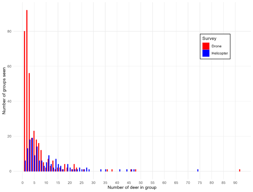
Figure 2: Bar graph of Deer group size distributions recorded by drone and helicopter surveys at North Arran
Click for a full description
Bars show the number of deer groups observed for each group size, for the drone (red) and helicopter (blue) survey. The x-axis shows the number of deer in a group, and the y-axis shows the number of groups of that size that were recorded. The data show that there were a greater number of small groups identified by drone.
Both surveys showed strong agreement in the spatial distribution of deer, with highest densities and concentrations in the north-east of the survey area, indicating that both surveys captured the same underlying population structure.
5.4.4 Interpreting the 300-Deer Discrepancy
The approximately 300-deer difference can be examined by considering the alternative hypotheses described in section 5.3.
Differences due to changes in abundance (Hypothesis 1) are unlikely. As described above, the population was expected to behave approximately as closed over the short interval between surveys. Those familiar with the site considered substantial movement from southern Arran over this period unlikely, and a change of this magnitude over one week is therefore implausible.
Differences due to incomplete spatial coverage (Hypothesis 2) may account for a small proportion of the discrepancy. In particular, conifer woodland, which comprises approximately 10% of the site, was excluded from both surveys. Deer using these areas would not be detected by either method and may move into and out of them between surveys. In principle, differences in the number of deer using conifer woodland between survey dates could contribute to differences in counts.
However, at this time of year most red deer on North Arran would be expected to use open hill habitats predominantly, except under adverse weather conditions. There was no evidence of such conditions during the surveys, suggesting that the number of deer using conifer woodland is unlikely to have differed substantially between surveys. Spatial coverage is therefore unlikely to explain more than a small proportion of the discrepancy.
There were also minor differences in areas covered by each survey. However, given the potential for movement between areas, these provide only limited evidence of the magnitude of any coverage-related difference.
Differences due to detectability (Hypothesis 3) provide the most plausible explanation. Detection from a helicopter using the naked eye depends partly on deer responding to disturbance by standing or moving. On Arran, deer appear relatively habituated to helicopter activity, likely due to frequent aviation associated with the nearby civilian airport and air ambulance or mountain rescue operations. As a result, deer may remain lying or stationary, particularly within vegetation cover, reducing visibility.
Vegetation further limits detectability. Both surveys were conducted when bracken and rhododendron provided substantial ground cover, within which deer may be partially or fully obscured from view from the helicopter. In contrast, the drone survey used thermal detection, which is less dependent on movement and less affected by vegetation structure, increasing the likelihood of detecting deer in such conditions. This suggests that some of the difference between counts is due to the detection method (naked eye vs thermal imager) rather than implicitly related to the use of a drone or helicopter.
Differences due to enumeration effects (Hypothesis 4) are considered unlikely to explain the discrepancy. The drone survey required substantial logistical effort, including two days of surveying with an east–west spatial split designed to minimise movement-related duplication. The split direction was chosen using local knowledge to reduce the likelihood of deer moving between survey blocks overnight. In addition, large groups observed at the end of Day 1 were relocated in imagery on Day 2, allowing high confidence in no duplication. Because helicopters group nearby deer together whereas drones identify smaller groups, differences in grouping between the two methods may contribute to variation in counts but are unlikely to account for a discrepancy of this magnitude.
Independent evidence from foot counts supports this interpretation. A coordinated foot count in May 2024 recorded 1,640 deer, and helicopter counts in 2014 were also lower than foot counts. Given expected recruitment between May and late summer, a late-August helicopter count would not be expected to fall below this level, unless deer consistently moved out of North Arran between May and September. However, this was not considered likely by survey managers familiar with the site. So, under-detection of helicopters rather than over-counting of drones and foot counts is considered more likely.
5.4.5 Interpretation
Given the largely closed population, especially with the short interval between surveys and the strong spatial agreement between methods the most plausible major explanation for the approximately 300-deer discrepancy is due to differences in the ability to detect deer. A key difference lies in the detection technology used, with thermal imaging compared to naked eye observation, in an area with substantial vegetation cover (bracken and rhododendron), and when deer have a reduced behavioural response to helicopter disturbance. Under these conditions, thermal imaging is more effective at detecting deer than visual observation alone. It is therefore likely that a helicopter survey using thermal imaging would detect more deer than one relying on visual observation alone.
Some contribution to the discrepancy from spatial coverage differences and local redistribution, in particular the conifer woodlands, are also possible, but these are unlikely to explain the majority of the difference.
Overall, this case study illustrates how substantial differences in estimated abundance can arise from observation-process variation, even under relatively stable ecological conditions and within the same landscape. This highlights the importance of explicitly considering detectability, either through survey methods that directly estimate detection probability or by understanding how factors such as vegetation, behaviour, and survey method influence when detection is likely to be high or low.
5.5 Case Study 2 – Duror–Glen Creran
The Duror–Glen Creran complex (Figure 3) provides a case study to compare quadcopter drone and helicopter survey methods in a heterogeneous woodland–open landscape. Unlike North Arran the two surveys covered different areas with only a small area of overlap.
5.5.1 State-process context
The Duror–Glen Creran complex represents a heterogeneous woodland–open mosaic landscape dominated by commercial conifer forestry, restock, broadleaved woodland, and open ground. Red deer are the dominant species, with roe deer also present.
The southern boundary of the drone survey area is largely unfenced, with known deer populations immediately to the south (as observed during the helicopter survey). Movement across this boundary is therefore expected, both seasonally and in response to disturbance or management. As a result, at the spatial scale of the surveys the population behaves as an open system (unlike North Arran), with substantial opportunity for movement within the wider FLS estate and into adjacent landscapes
In addition, 11 red deer and one roe deer were culled in the 13 days between the drone survey and the helicopter survey (although this is small compared to the overall number of deer in the area). Together with the movement these factors mean that true abundance within the survey area could have changed between surveys, and that redistribution is likely to have occurred.
As a result, this case study does not provide a clean test of observation processes alone, but instead illustrates how state-process dynamics, boundaries, and openness complicate method comparison.
5.5.2 Observation-process context
The quadcopter drone survey was conducted over three days (5 – 7 March 2024), with two operators to cover the entire Duror-Glen Creran FLS site complex (an area of 97km2) . In contrast, the helicopter survey, conducted on 20 March 2024, covered the southern open hill portion of the Duror-Glen Creran complex, together with additional open ground to the south beyond the FLS boundary (an estimated area of 235km2) (see Figure 3).
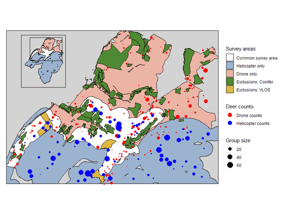
Figure 3 Map of the Duror–Glen Creran survey site showing survey coverage, exclusion areas, and deer observations.
Click for a full description
Scaled points indicate group sizes of 20, 40 and 60 in the location of deer groups recorded by quadcopter drone (red) and helicopter (blue). Areas surveyed only by drone are shown in red, areas surveyed only by helicopter are shown in blue, and the common survey area, used for population comparisons in white. Exclusion areas include conifer woodland (green) and areas outside the drone visual line of sight (VLOS) (yellow); VLOS exclusions apply only to the drone survey. Helicopter survey boundaries are estimated from flight paths. The inset shows the full extent of the helicopter and drone survey areas; the rectangle indicates the area enlarged in the main panel.
The drone survey included a substantial number of exclusion zones, primarily due to dense conifer canopy and visual line-of-sight (VLOS) constraints. Whilst the VLOS constraints are only applicable to the drone, dense conifer canopy limits detectability for both survey methods. Although not explicitly mapped for the helicopter survey, it is assumed that these areas were also effectively excluded, as deer within dense conifer would not be visible.
The helicopter survey area used for comparison was reconstructed based mainly on forestry boundaries and observed flight coverage and should therefore be considered an informed approximation of the survey area covered rather than an exact footprint. This is particularly the case in defining the overlap between surveys, and along the northern boundary and parts of the eastern and western edges of the site.
5.5.3 Results and direct comparison
The spatial overlap between the two surveys has an area of 34 km² (Figure 3). Of this, 4.5 km² was excluded due to dense conifer from both surveys. An additional 2.4 km² was excluded from the drone survey due to loss of VLOS. Since this survey, more portable quadcopter models would mean that many of these areas lost to VLOS could be reached on foot.
In total, considering only the area surveyed in both methods, the helicopter survey recorded 448 red deer (a density of 16.6 per km2) and the drone survey 386 red deer (a density of 14.3 per km2). This is a difference of 62 deer (14%) of the helicopter count.
Extrapolation beyond the surveyed area is not considered appropriate because deer densities are expected to be different within the coniferous woodlands compared to the surveyed areas.
5.5.4 Interpreting differences: hypotheses mapped to state and observation processes
The hypotheses set out in Section 5.3 are used to evaluate possible reasons for the difference of over 100 deer in the population total.
Differences due to changes in the state process (Hypothesis 1) are likely to be the dominant explanation. In contrast to North Arran, the population behaves as an open system at the spatial scale of the surveys, with movement into and out of the survey area expected. The presence of deer to the south of the common overlap area (Figure 3) and the lack of strong boundary features mean that animals may move into or out of the common survey area between survey dates. In addition, culling that occurred between surveys (and between days of the drone survey), may contribute directly to changes in abundance (on a small scale) and indirectly through disturbance. As a result, differences between population totals may reflect real changes in the number of deer present within the surveyed area at the time of each survey, rather than because of the differences in the survey methods.
There is also likely to be some contribution from observation-process effects, although their individual influence is more difficult to isolate given that the surveys do not cover identical areas.
Considering spatial coverage (Hypothesis 2), approximately 16% of the overlap area, comprising dense conifer, was not surveyed by either method. Deer using these areas may move into and out of the surveyed area between surveys. In contrast to North Arran, this effect may be more important because it represents a larger proportion of the site, surveys were conducted under less favourable weather conditions, and the unsurveyed areas are often located along site boundaries rather than within the interior. As a result, deer moving into these areas may leave the survey area entirely, whereas in North Arran deer not in conifer woodland were still largely within the surveyed system. However, the magnitude of this effect is difficult to determine. In addition, the areas surveyed differed between methods, and deer were observed in areas excluded from the drone survey due to VLOS constraints, indicating that animals were present in parts of the site not consistently covered.
In terms of detectability (Hypothesis 3), its effect is more difficult to interpret. As in North Arran, detection would generally be expected to be higher using thermal imaging than naked eye observation, which would tend to increase counts from the drone survey. However, the effects of vegetation and reduced behavioural response to helicopters may be less pronounced in this case. At the same time, helicopter disturbance may flush deer from woodland and edge habitats, altering their distribution during the survey. The net effect of detectability is therefore unclear.
Enumeration effects (Hypothesis 4) are considered unlikely to explain the discrepancy between surveys given the survey protocols in place.
5.5.5 Interpretation and value of this case study
This case study demonstrates the limits of direct numerical comparison between survey methods where the population changes substantially between surveys due to the state process. Here, differences between quadcopter drone and helicopter results are likely to reflect a combination of real population change and redistribution, movement across weak or unfenced boundaries, culling-related disturbance, as well as observation process issues such as incomplete and non-overlapping coverage, and detectability limitations in dense forestry.
While this makes Duror-Glen Creran unsuitable for a strict comparison of different survey methods, it reflects the situation described in Chapter 3 for open populations and illustrates how population openness, species characteristics, habitat structure, and boundary definition can shape survey interpretation in many real-world forestry landscapes. In such settings, population totals within the area covered by both surveys may reflect site use over short periods rather than stable local population size. As a result, the concept of a true population size becomes less meaningful, as movement dominates variation in counts, making it difficult to both detect genuine population change or to compare survey methods.
5.6 Results in the literature
Empirical comparisons between deer survey methods are uncommon, largely because true abundance is rarely known and because differences between estimates can reflect both state-process variation (movement and redistribution between surveys) and observation-process limitations (coverage, detectability, and inference). The most directly relevant Scottish evidence base is therefore work that compares methods by repeating surveys over short intervals and assessing variation and operational performance rather than “accuracy” against a known truth.
5.6.1 Direct Scottish comparison: Daniels (2006) open-range red deer
Daniels (2006) provides one of the clearest Scotland-focused comparisons of survey methods for open hill red deer. Four approaches – ground counts, visual helicopter counts, infrared helicopter counts, and dung counting – were compared across three sites (Syre, Croggan/Laggan, and Rum) during late winters 2003–2005. Because true population totals were unknown, performance was assessed through repeatability (precision), expressed as coefficients of variation (CV) from repeat counts conducted close together in time, when deer movement is typically reduced. Across sites and methods, within-method CVs ranged from approximately 5–16%, with ground and visual helicopter counts showing the lowest variation in total counts. Infrared surveys were limited by the rarity of suitable Scottish conditions.
Within the framework developed in Chapters 3 and 4, the state process in Daniels most closely resembles a Strathconon-type system, where surveys aim to encompass most routine movement, but complete closure is not achieved. Short-interval variation arose from three sources that map directly onto the framework. First, movement across porous boundaries and weather-driven redistribution altered the number of animals available to be counted, representing state-process variability. Second, differences in routes or flight paths changed the extent of “dead ground”, areas that were not surveyed, reducing spatial coverage and leading to variation in the amount of spatial coverage. Third, observer differences in spotting, counting, and classifying deer affected detectability and enumeration. Furthermore, visual estimation underestimated large group sizes, and that re-counting large aggregations using digital photography improved accuracy.
In all cases the helicopter surveys were often the least labour-intensive, and in two out of three sites the most cost-effective method.
Overall, all surveys were conducted under near “best case” conditions in large upland areas with relatively closed populations and areas small enough to be covered rapidly. Recommendations such as standardising routes and observers and using photography were measures that reduced observation-process variability and improve comparability over time. This work has since informed best practice for these different methods.
5.6.2 Broader comparative evidence: what general studies add (and what they do not)
Beyond Daniels (2006), relatively few studies provide direct, same-site comparisons of multiple deer survey methods that include at least two of the survey methods considered in this report.
Marcon et al. (2019) compared foot counts (drive counts undertaken at sampled locations), dung surveys (using FAR approach) and camera trapping (using REM) for roe deer in a mountainous study area in the Casentino Valley, Italy. Dung surveys produced the most precise estimates and required fewer personnel, foot counts were the least precise and most labour-intensive, with camera trapping in between these. However, the methods were not applied at the same time, limiting direct comparability.
Pfeffer et al. (2018) compared dung surveys (a form of FAR) and camera trapping (REM) for roe, red and fallow deer within a forest–agriculture landscape in southern Sweden that was relatively closed (bounded by sea and infrastructure). Both methods were applied over a comparable time period. Density estimates differed between methods, with dung surveys combining roe and fallow deer, while camera trapping allowed species-level estimates but was sensitive to different parameterisations of the REM.
Comparisons involving UAV surveys are particularly limited and generally not directly applicable to the quadcopter-based thermal methodology considered here. For example, McMahon et al. (2021) used a fixed-wing UAV with transect-based sampling and image processing to detect individuals, while Paulsen et al. (2023) used optical (RGB) imagery in strip transects rather than thermal sensors. Both approaches differ substantially in survey design and detectability from the UAV methodology considered in this report and therefore provide limited basis for direct comparison with other methods.
Overall, there is further work needed to compare these different methodologies.
6. Comparisons of Resource Requirements
6.1 Purpose and Scope of Resource Comparison
Survey method selection cannot be determined solely by statistical performance. Methods must also be operationally feasible, repeatable over time, and sustainable within operational resources, workforce, and environmental constraints. In practice, the most statistically robust method is not necessarily the most deliverable at landscape or national scale.
This chapter develops a structured framework for comparing survey methods across environmental (carbon) cost and key operational drivers. Carbon is used as the organising baseline because it can be quantified consistently across methods and scenarios using standardised emission factors. Alongside this, the chapter considers different operational factors and Table 5 provides a summary of equipment, workforce requirements, time to delivery, and data processing demands associated with each method. A full financial costing is beyond the scope of this assessment.
The six sites illustrating the scenarios described in Chapter 3 are used as comparative case studies. Drone surveys have been carbon costed in full across all six scenarios. Three scenarios – Strathconon (remote open hill), Torrachilty (upland forestry), and Devilla (accessible lowland forestry) – are used for cross-method comparison of carbon costs based on operational resource requirements. These sites represent contrasting logistical and ecological contexts, ranging from remote and extensive to more accessible and spatially compact. Not all methods are suitable across all landscapes and resource demands (and therefore carbon cost) may scale differently across methods and sites. Together, the three sites provide a structured basis for examining how environmental impact and resource demands vary according to both landscape and method.
6.2 Environmental (Carbon) Costing Framework
6.2.1 Accounting principles and scope
Environmental costs were calculated following NatureScot guidance using the UK Government Greenhouse Gas (GHG) Conversion Factors for Company Reporting (2025).
The assessment primarily reflects Scope 3 emissions, representing contracted survey activity. These include the key sources of emissions associated with carrying out surveys including travel, overnight accommodation and office-based activities. These are defined in more detail in Section 6.2.2.
Scope 2 emissions, for example those associated with equipment manufacture, software development, and end-of-life disposal were excluded, as the objective is to compare operational costs, from NatureScot commissioning a survey, rather than infrastructure investment (for example the buying of quadcopter drones or cameras for camera trapping) needed for NatureScot to do the whole survey in-house.
In addition, helicopter aviation fuel, which constitutes Scope 1 emissions, were required reflecting direct fuel combustion.
6.2.2 Standardised cost components
To allow consistent comparison across survey approaches, carbon costs were calculated using a common set of components which translate the accounting scope described above into measurable elements.
Planning and processing covered pre-survey planning, on-the-day coordination, and post-survey data processing, analysis and reporting. These activities are assumed to be undertaken from office or home working locations.
Travel to site includes the movement of personnel and equipment between the contractor base and the survey location. For the purposes of comparison, all sites were assumed to be 100km away from the contractor base. Except for the helicopter survey, transport was assumed to be a large diesel-powered ‘pick-up’ type vehicle (e.g. a 4WD) as this was needed to carry equipment and/or move around the site. The number depended on the logistics of each survey. Where estate staff might typically be employed to carry out the survey (such as foot surveys or vehicle-based distance sampling), the travel costs for these staff were assumed to be zero. In all cases, survey design and delivery were assumed to minimise the number of vehicles and overall travel requirements, so that estimates reflect an efficient but realistic implementation of each method.
Travel within site includes all vehicle movement within the site to complete the survey and varies depending on terrain and access (e.g. helicopter, diesel vehicle, ATV, or foot access). For quadcopter drone surveys, on-site travel was derived from a mapped route linking all flight locations, Equivalent or scaled versions of these routes were then used to estimate the within-site travel for other survey methods.
When surveys extended beyond one day, accommodation for overnight stays was included for each surveyor.
Finally, operational costs such as electricity for charging quadcopter drone batteries was included. No costs were included for charging of equipment used across all methods – such as navigation, cameras or communication tools.
Carbon costs associated with data storage and image processing have not been included, as these are not directly represented within the standard emissions factors used. However, this warrants further investigation in the future.
6.3 Quadcopter Drone Carbon Results Across Landscape Scenarios
Quadcopter drone surveys were costed in detail across six landscape scenarios and provide the baseline for environmental comparison. The survey planning and time required was based on BH Wildlife Consultancy’s experience of drone surveys, in many cases, at the sites in question.
Survey planning included identifying the locations from which the drone could be flown to ensure complete coverage of the site. On-site travel consisted of mapping the route around the site to ensure all flight points were visited. Each drone operator travelled in a separate vehicle and on-site travel was calculated as the total distance to visit all flight points multiplied by the number of vehicles. Between one and four drone operators survey a site.
Processing and reporting time is relatively short because BH Wildlife Consultancy has invested in developing a data pipeline that enables efficient transfer of data from the field directly into Geographic Information Systems (GIS) and rapid report production.
The outputs from the drone surveys include the number of deer seen on the site, the minimum counts, disaggregated by species, and where possible sex and age, maps indicating the locations of all groups observed and parts of the site that were not surveyed.
6.3.1 Total emissions across scenarios
Table 3 gives the estimated total emissions per site in kgCO2e. The cost per km is calculated first for the total carbon cost and secondly omitting travel to the site.
| Site | Area km2 | Office Total | On site Battery | On site Over night | On site Travel | On site Total | Travel to site | Overall Total | Cost per km2 Total | Cost per km2 No travel |
|---|---|---|---|---|---|---|---|---|---|---|
Strathconon | 375 | 8.0 | 7.6 | 125 | 20 | 153 | 164 | 325 | 0.9 | 0.4 |
Torrachilty | 77 | 8.0 | 3.2 | 21 | 23 | 47 | 84 | 139 | 1.8 | 0.7 |
Easterhouse | 7 | 4.0 | 0.5 | 0 | 5 | 5 | 42 | 51 | 7.3 | 1.3 |
Devilla | 8 | 4.0 | 0.7 | 0 | 3 | 4 | 42 | 50 | 6.3 | 1.0 |
Arable | 3 | 4.0 | 0.1 | 0 | 1 | 1 | 42 | 47 | 15.6 | 1.7 |
Craigellachie | 2 | 4.0 | 0.3 | 0 | 0 | 0 | 42 | 46 | 23.0 | 2.0 |
Carbon emissions increase with the size of the site but not in direct proportion to survey area. Strathconon – the largest site – had the largest carbon costs of 325 kgCO2e and Craigellachie – the smallest site – the lowest 46 kgCO2e.
Across all scenarios the largest contributor to emissions was travel to the site. It is especially worth noting that at Craigellachie, where travel round the site is on foot, around 91% of the carbon costs comes from the travel to the site. If we had assumed a different travel distance to the site, the overall carbon costs would be different although the ordering between sites would be the same.
Where surveys required more than one day of fieldwork (Strathconon and Torrachilty), accommodation became a major additional contributor to the carbon cost. For example, Strathconon, which was a large survey, required three nights’ accommodation for each of four surveyors.
Other components contributed comparatively less to the sites. On-site travel varies with terrain and survey duration but was always secondary to travel to site. Electricity consumption for quadcopter drone battery charging represented only a small proportion of total emissions.
For the smaller sites (Devilla, Easterhouse, Arable and Craigellachie) carbon costs were similar. This reflected the single-day deployment, minimal personnel and no accommodation. In these cases, the costs of office work in planning, analysis and report writing were similar or more than the cost of travel round the site.
These fixed costs meant that the carbon costs overall did not scale with area. Even so, the carbon cost per km2 decreased with the size of the site, even when the cost of travelling to the site was excluded.
6.4 Extending the Framework to Other Survey Methods
This section extends the carbon costing framework to other survey methods, examining how carbon emissions vary across the three selected sites of Strathconon, Torrachilty and Devilla. These sites are intended to illustrate how carbon costs vary with landscape type, survey duration, and operational requirements, as can be seen from the costing of the drone surveys. Not all survey methods are applicable across all sites, so they were only included where they were operationally realistic. Estimates are based on a combination of recent survey delivery, existing reports, and indicative assumptions where direct data were not available. Details are provided in Table 4.
| Method | Site | Office Days Pre-survey | Office Days Post-survey | personnel per visit Local1 | personnel per visit External2 | visits | days per visit | Over night stay needed | Travel On-site | Travel To/from site | Survey effort | Additional Information |
|---|---|---|---|---|---|---|---|---|---|---|---|---|
| Helicopter | Strathconon | 1 | 4.75 | 63 | 74 | 1 | 1 | No | 2 x helicopter | 2 x helicopter | 12 hours + 12 mins flying | 160 L/hr fuel |
| Drone | Strathconon | 1 | 2 | 0 | 4 | 1 | 3 | Yes | 4 x ATV | 4 x pick-up | Flight points5 | Batteries for 4 drones6 |
| Drone | Torrachilty | 1 | 2 | 0 | 2 | 1 | 2 | Yes | 2 x pick-up | 2 x pick-up | Flight points | Batteries for 2 drones |
| Drone | Devilla | 0.5 | 1 | 0 | 1 | 1 | 1 | No | 1 x pick-up | 1 x pick-up | Flight points | Batteries for 1 drone |
| Foot | Strathconon | 1.5 | 3 | 10 | 6 | 1 | 2 | No | 13 x pick-up | 4 x pick-up | Full ground sweep | - |
| Dung | Torrachilty | 2 | 7 | 0 | 4 | 2 | 3 + 67 | Yes | 2 x pick-up | 2 x pick-up | 45 FAR + 90 FSC8 | - |
| Dung | Devilla | 2 | 4 | 0 | 4 | 2 | 2 + 1.59 | Yes | 1 x pick-up | 1 x pick-up | 49 FAR transects10 | - |
| Camera | Torrachilty | 1 | 5 | 0 | 1 | 3 | 6 + 2 + 3 | Yes | 1 x pick-up | 1 x pick-up | 75 cameras | - |
| Camera | Devilla | 1 | 2 | 0 | 1 | 3 | 1 + 1 + 1 | No | 1 x pick-up | 1 x pick-up | 15 cameras | - |
| Vehicle-based distance | Devilla | 0.5 | 1 | 2 | 0 | 1 | 2 | No | 1 x pick-up | 1 x pick-up | Night transects (18.5km) | - |
Footnotes
1 Local staff are those that are employed by the estate
2 External staff are not employed by the estate
3 One per helicopter and four driving on ground
4 Two x (pilot, navigator, observer) plus driver of fuel bowser
5 Distance needed to visit all flight points
6 Drones available are three M30 and one M350, Each has nine sets of batteries that need charging each day
7 Assume each surveyor does four plots per day first visit and six plots per day second visit
8 Similar number of pots to last dung survey and ratio of FAR:FSC of 1:2 is similar to other FLS sites.
9 Assume each surveyor does six plots per day first visit and eight plots per day second visit as close together
10 Same number of plots as last dung survey
6.4.1 Helicopter surveys
Carbon costs for a helicopter survey were only estimated for Strathconon; this was the only site where this method was operationally relevant. Estimates were based on a recent survey undertaken there, which used two helicopters over a single day. Emissions from the helicopter were calculated from total flight time, including travel to and from the site and time spent surveying, and converting to fuel use using a standard litres-per-hour value.
Each helicopter carried a pilot and three observers with one drawn from estate staff. Travel to the site was included for the non-local personnel, along with the movement of a fuel bowser and support vehicle required for refuelling operations. Travel to the site for helicopters, personnel and support vehicles was calculated using the standardised 100km distance assumption described in section 6.2. It was assumed that a helicopter took 40 minutes to fly 100km.
Outputs include minimum count of the number of red deer on the site with sex and age where possible, map locations and outputs on the NatureScot website.
6.4.2 Foot survey
Carbon costs for foot surveys were estimated for Strathconon only, based on resource information provided by the estate manager (Masson, pers. Comm.) on previous surveys undertaken at the site.
The survey was carried out by a combination of estate staff, for which no travel was considered, and locally based surveyors, for which estimates of actual travel distance were provided. It took place over two days, but because staff were local no accommodation costs were assumed. Movement within the site was based on the distance used by drone operators to move around the site for each of the vehicles deployed.
A comparison scenario in which all non-estate surveyors travelled the standard 100km each way, and required overnight accommodation was also considered.
Outputs were a minimum count of the number of red deer on the site with sex and age where possible and map of locations.
6.4.3 Vehicle-based distance sampling
Vehicle-based surveys will be considered for Devilla only, where terrain and access make this method operationally feasible. Estimates are based on indicative assumptions regarding survey design, transect length, and staffing, informed by practitioner input based on woodland surveys carried out in England (e.g. Forest of Dean).
The survey is assumed to be undertaken using a single ‘pick-up’ type vehicle over two nights using two estate staff – a driver and a recorder/observer. As staff are local, travel-to-site emissions and over-night accommodation are not required. A comparison scenario in which surveyors travel from further afield, based on the standardised 100 km distance assumption and overnight accommodation, was also considered. Movement within the site is based on the estimated length of survey transects.
The output is an estimate of the population total derived from standard distance sampling methods. It was not clear whether sufficient data would be available to disaggregate the data by sex and age. A spatial map of deer distribution could also be produced by fitting appropriate models, although this would require additional analysis.
6.4.4 Dung surveys
Carbon costs for dung surveys were estimated for Devilla and Torrachilty based on FLS dung survey reports from these sites and others to guide transect density, published guidance on survey timing, and site-specific assumptions regarding field effort. Equivalent estimates were not developed for Strathconon due to the absence of comparable survey reports.
The FAR survey methodology was assumed, meaning sites were visited twice (with a gap of several weeks), so as to be able to estimate dung accumulation directly. At Devilla, all plots were surveyed during each visit, whereas at Torrachilty only a third of transects were FAR transects, that is they were surveyed during both visits. This was deemed sufficient to estimate dung accumulation rates. The rest were FSC transects and were only surveyed on the second visit. Number of person days required to survey the sites was estimated based on typical plot completion rates (Swanson et al 2008) with an adjustment for Devilla as the site was small and plots were close together.
Field teams were assumed to consist of four surveyors. Distances travelled round the site was a multiplier of 1.25 times the equivalent drone survey distance. This reflects the need to transport multiple surveyors, including additional travel to drop off and collect surveyors and the greater number of transects relate to drone flight points.
Estimates therefore include repeated travel to site, movement within the site during each visit, and, where required, overnight accommodation for survey teams.
Time for office-based activities assumed that data were recorded in the field on paper and subsequently transferred into digital format, as was our understanding for the FLS surveys carried out around 2022. These estimates are approximate and effort may be reduced if digital data collection methods were used.
The FLS reports provided detailed outputs which included the use of additional data, such as cull records, to inform population modelling and advice on setting cull quotas. For the purposes of this comparison, a reduced level of analysis was assumed focusing on the production of population estimates only.
6.4.5 Camera trapping
Carbon costs for camera trapping were estimated for Devilla and Torrachilty based on discussions with practitioners and indicative assumptions regarding survey design, camera density, and deployment strategy. These estimates are more uncertain than for other methods, as they are not based on past surveys at these sites. In contrast to other survey approaches considered here, camera trapping does not currently have a well-established standard methodology for deer in the UK or Scotland, and survey design can vary substantially depending on the approach taken. As a result, both the resource requirements and the precision of resulting estimates may vary widely.
As described in Chapter 4, the assumed methodology was the Random Encounter Model using motion-sensitive cameras. Three visits to the site were assumed for installation, checking, and retrieval spaced over six weeks or more. The ratio of cameras to area differed at the two sites because of the different species, and their different home ranges. Field effort was based on a single surveyor, with estimates of time derived from experience in other parts of the UK.
Movement within the site was assumed to follow similar routes to those used for drone surveys. Estimates therefore include repeated travel to site, movement within the site on each visit, and, where required, overnight accommodation for the surveyor.
Data processing and analysis was based on manual assessment of images. To calculate estimates additional information and multipliers are required. Here, these are assumed to be calculated from the literature rather than being collected as part of the study which would increase the accuracy of results but also the time needed in the field. Thus, this is very much a minimum carbon cost.
An alternative camera-based approach, currently being proposed at another big site (527km2) elsewhere in Scotland for NatureScot, was also considered. This approach used cameras that captured an image every 5 minutes. This results in substantially larger data volumes and so the image analysis is automated. A large number of cameras is needed to cover this big site, so only part of the site is surveyed at one time and the cameras then moved to survey the rest. This requires an additional two site visits. A carbon cost was calculated for this survey using the estimated timings for this proposal. This was not included in the main comparison tables but is noted separately for reference.
Outputs from camera trap surveys include estimates of deer numbers, disaggregated by sex and age depending on survey design and data quality.
6.5 Results
Tables 5-7 show the number of kilogrammes of carbon dioxide CO2e associated with different census methods for each site. The Calculation Basis column represents the quality of the estimate, with A indicating results come from actual surveys at the site, B indicating estimates are derived from site-specific reports, and C more indicative or assumption-based estimates.
6.5.1 Strathconon - 375 km2
| Method | Calculation basis | Office pre & post | On site Battery | On site Over night | On site Travel | On site Total | Travel to site | Overall Total | Total carbon cost per km2 | Total carbon cost per km2 No travel |
|---|---|---|---|---|---|---|---|---|---|---|
| Helicopter | A: Survey | 16 | 0 | 0 | 4968 | 4968 | 1157 | 6141 | 16.4 | 13.2 |
| Drone | A: Survey | 8 | 8 | 125 | 20 | 153 | 164 | 325 | 0.9 | 0.4 |
| Foot (local) | A: Survey | 12 | 0 | 0 | 96 | 96 | 0 | 108 | 0.3 | 0.3 |
| Foot | A: Survey | 12 | 0 | 114 | 96 | 210 | 336 | 558 | 1.5 | 0.6 |
All three estimates for Strathconon were derived from actual surveys carried out at the site providing a robust basis for comparison.
The helicopter survey had by far the highest carbon cost (6141 kgCO2e), driven by the carbon cost of aviation fuel (over 98% of the total). This was approximately twenty times higher than the carbon cost of the drone survey (325 kgCO2e). The foot survey (assuming local staff) had the lowest carbon cost (108 kgCO2e). However, when most surveyors are assumed to travel to the site the carbon cost increases substantially, becoming around five times higher than the drone survey. Even under this assumption the foot survey remains approximately twelve times lower than the helicopter survey. As an aside, a rough calculation for the proposed large NatureScot survey using camera traps at a site of 527km2 with five visits came to a cost of around 650kgCO2e.
6.5.2 Torrachilty - 77km2
| Method | Calculation basis | Office pre & post | On site battery | On site over night | On site travel | On site total | Travel to site | Overall total | Carbon cost per km2 Total | Carbon cost per km2 No travel |
|---|---|---|---|---|---|---|---|---|---|---|
| Dung | B: Reports | 24 | 0 | 291 | 58 | 349 | 168 | 541 | 7.0 | 4.8 |
| Camera | C: Assumptions | 16 | 0 | 83 | 35 | 118 | 126 | 260 | 3.4 | 1.7 |
| Drone | A: Survey | 8 | 3 | 21 | 23 | 47 | 84 | 139 | 1.8 | 0.7 |
Unlike Strathconon, only the drone survey estimate was directly based on a survey, with the dung survey estimates based on FLS reports and literature and the camera trapping estimates are indicative.
At this site, the dung survey (541 kgCO2e) had approximately twice the carbon cost of the camera survey (260 kgCO2e) and nearly four times the carbon cost of the drone survey (139 kgCO2e). The high cost of the dung survey is primarily due to accommodation (291 kg CO2e) because of the need for multiple surveyors over several days in each of two separate visits. The two visits are needed to be able to calculate one of the multipliers (pellet persistence or accumulation rate) directly in the field. Although the camera trapping survey required an additional visit to the site compared to the dung survey this was offset by using only a single surveyor and vehicle. However, these camera trap estimates are sensitive to survey design assumptions. For example, approaches that estimate additional multipliers parameters (such as animal movement rates), rather than using values from the literature, may make this more comparable with the dung surveys. This will increase time on site, processing requirements and overall carbon cost as well as precision and accuracy of the estimates.
6.5.3 Devilla - 8km2
| Method | Calculation basis | Office pre & post | On site battery | On site over night | On site travel | On site Total | Travel to site | Overall Total | Total carbon cost per km2 | No travel carbon cost per km2 |
|---|---|---|---|---|---|---|---|---|---|---|
| Camera | C: Assumptions | 8 | 0 | 0 | 10 | 10 | 126 | 144 | 18.0 | 2.3 |
| Dung | B: Reports | 19 | 0 | 0 | 9 | 9 | 84 | 112 | 14.0 | 3.5 |
| Drone | A: Survey | 4 | 1 | 0 | 3 | 4 | 42 | 50 | 6.3 | 1.0 |
| Vehicle (local) | C: Assumptions | 4 | 0 | 0 | 4 | 4 | 0 | 8 | 1.0 | 1.0 |
| Vehicle | C: Assumptions | 4 | 0 | 21 | 4 | 25 | 42 | 71 | 8.8 | 3.6 |
Only the drone survey estimates were based on actual surveys with dung survey estimates based on reports and the vehicle and camera trapping estimates are assumption based.
Because Devilla is a relatively small site, all, except the vehicle-based survey were completed in a single day even if the number of surveyors varied on the site (for example dung surveys still required multiple surveyors). As a result, travel to the site, is the dominant contributor to the carbon cost across methods. The relative size of total carbon cost is proportionate to the number of visits.
The camera trapping study had the highest carbon cost (144 kgCO2e), reflecting the need for three separate visits to the site. In contrast, the dung survey required two visits resulting in a lower overall cost (111 kg CO2e) and the drone a lower cost (50 kg CO2e) still, as this was one visit. The vehicle-based distance sampling had the lowest carbon cost (assuming locally based staff) (8 kgCO2e). With non-local staff the cost increases (71 kgCO2e) because it requires accommodation for three staff.
6.6 Integrated results and interpretation
This section brings together the results to highlight the key factors influencing carbon cost, operational requirements and survey outputs across methods.
6.6.1 Carbon costs
The most immediate distinction is that the high carbon cost of aviation fuel means that helicopter surveys are an order of magnitude more expensive than any other survey method. Even travelling 100km to reach a site by helicopter has a carbon cost around 12 times higher than a large diesel vehicle. This is before accounting for the flight time (and therefore carbon cost) needed to survey the whole site. In helicopter surveys, this high carbon cost is intrinsic to achieving full site coverage. In contrast, other methods that aim to achieve full coverage (such as quadcopters or foot-based approaches) have very low carbon costs associated with the survey itself, with vehicles used only to move personnel and equipment rather than to provide coverage.
For all other survey methods, travel to the site is the major driver of emissions across all scenarios, although this clearly depends on the actual distance between the site and the surveyors’ base. The number of trips to the site, whether over time or multiple vehicles at the same time, strongly influences the overall environmental impact of a survey. Multi-day surveys, particularly those with multiple surveyors, introduce substantial additional emissions through accommodation. In our scenarios, the carbon cost of accommodation per surveyor is around four times lower than the 200km round trip in a large diesel vehicle. Methods that can be delivered in a single visit (drones or vehicle-based surveys) or within a single day therefore have the lowest carbon costs. The use of local survey teams, reducing both travel costs and overnight stays, will significantly reduce carbon cost.
For small sites, fixed logistical costs form a larger proportion of total emissions, meaning that carbon cost per unit area is higher than for larger sites. Where feasible, combining nearby survey areas within a single deployment may reduce carbon cost per unit area. One caveat to this is that in all these scenarios the site belonged to one landowner. When multiple landowners are involved additional planning effort is required, which may offset some of these gains, although the overall effect on carbon cost is likely to be small unless travel distances or low or the number of landowners very large.
For sampling-based methods, increasing sampling intensity improves the precision of estimates but also increases survey effort and associated carbon cost. The same is true for methods that estimate additional parameters, or multipliers, such as for dung and camera surveys. There is therefore a trade-off between statistical confidence and environmental cost.
6.6.2 Operational requirements
Table 8 summarises the key resources including people skills, time, equipment and data, and main outputs for each survey method
| Method | Planning & Design Requirements | Field Roles & Effort | Field Time Requirement | Field Equipment | Processing & Analysis Workload | Typical Data Volume | Typical Outputs |
|---|---|---|---|---|---|---|---|
| Helicopter aerial count | Flight route planning Aviation permissions Weather coordination | Licensed helicopter pilot Trained aerial observers Ground support (fuel bowser/4WD) | Single survey period Rapid full-site coverage | Helicopter hire Aviation fuel & Fuel bowser 4WD support vehicle GPS & recording device Camera Communications between helicopters | Image Review for id, double count & enumeration Manual Summaries GIS mapping & data management | Mb-GBs | Typically, red deer; Total abundance (minimum count & density) Disaggregated by sex & age Group location (group size, sex & age) |
| Quadcopter (thermal/RGB) | Survey design Flight planning CAA compliance Battery/logistics planning | Licensed UAV pilot One or more depending on site | Single survey period May require multiple days | 1–10 kg UAV with thermal, RGB & zoom cameras Ground station Batteries Communication between pilots GPS & Recording device GIS & processing software | Image Review for id, double count & enumeration GIS mapping & data management | 10s–100s GB | All deer species; Total abundance (minimum count & density) Disaggregated by species, sex & age Group location (species, group size, sex & age) |
| Foot (ground) count | Survey route planning Coverage allocation | Trained ground observers & coordinators | Single survey period Ideally all in one day | Optics (binoculars/spotting scope) Radio communication between foot teams GPS & recording device | Data collation and summary | KB | Typically, red deer Total abundance (minimum count & density) Disaggregated by species, sex & age Group location (coarse - potentially by zone) (group size, sex & age (where possible)) |
| Vehicle-based survey with distance sampling | Route & sampling strategy design (including distance sampling considerations) | Driver Thermal operator | Single survey period Often multiple nights | Vehicle Thermal imager Optics Angleboard Communication between vehicles GPS & recording device | Distance sampling statistical modelling Potentially spatial modelling | MB–GB | All deer species Density estimate and total with confidence interval. Potential for spatial modelling Disaggregated by species Sample transects - group location (group size, species sex & age) |
| Dung count (pellet group count) | Sampling design (transects) Calibration decisions Repeat-visit schedule | Trained field surveyors | Multiple visits (clearance + recount) Several weeks/months between visits. | Plot markers GPS & recording device | Sample estimation Calibration to convert pellets to density | MB | Red deer & other species combined Site use/density estimate and total with confidence interval Disaggregated by red or other deer species Sample points (deer utilisation potentially by red & other species) |
| Camera trap survey (REM) | Deployment design Calibration decisions | Field staff for installation, maintenance, retrieval | Multiple visits (deployment, battery/SD changes, retrieval) | Camera traps Batteries SD cards Mounts Data storage & processing software | Large image datasets classification (manual or AI) Database management Statistical modelling for density | 10s–100s GB (or more) | All deer species Site use/density estimate & total with confidence interval Disaggregated by species (and potentially sex, age) Sample locations (species presence, activity patterns) |
6.6.2.1 Field delivery: people and equipment
Survey methods differ considerably in the number of personnel required and the level of specialist expertise involved, which can be linked to the type of equipment required. In all cases, appropriate training and access to equipment are essential to ensure that surveys are carried out consistently and that results are not biased or imprecise.
Methods requiring licensed operators, such as helicopter and quadcopter surveys, may be constrained by workforce availability. In contrast, approaches such as dung surveys and foot counts rely on larger numbers of field staff deployed over several days.
In practice, dung surveys are typically undertaken by trained surveyors, whereas foot counts (and distance sampling) may rely on locally available staff (as assumed in the scenarios considered here). Where this is not possible, contracted surveyors may be required, with implications for both cost and carbon through additional travel and accommodation.
There are also important differences in the balance between field effort and technical capability. Methods involving aerial platforms or camera systems require investment in equipment, software and supporting systems, including UAV platforms, sensors, camera units and data processing tools. Ground-based approaches require less specialised equipment but may involve more extensive field deployment and coordination.
All survey methods require in-field recording systems, now typically GPS-enabled devices, and reliable communication between teams where multiple observers or platforms are involved to ensure coordinated coverage and help avoid double counting.
6.6.2.2 Data processing and analysis
Survey methods generate markedly different data types and volumes. Drone and camera surveys produce large image datasets, while helicopter surveys may also generate high-resolution imagery. In contrast, foot counts produce small volumes of observational records with relatively low data storage requirements, while distance sampling and dung surveys generate sampled ecological data requiring structured recording and subsequent analysis.
Skills in GIS (for all methods except foot surveys), survey design (for sample-based methods), and statistical modelling (distance sampling, dung surveys and camera trapping) are required to translate field observations into robust estimates.
Data processing intensity contributes to environmental and operational costs through computing, storage and analytical time. Image-based methods in particular require classification, quality control and integration into outputs, and may become a bottleneck where large volumes of data are generated. This is especially the case for camera trapping surveys, where image processing demand can be substantial, and may be substantially higher if continuous use (e.g. every five minutes) image capture is used instead of motion-triggered cameras.
A detailed assessment of the environmental and financial costs associated with data processing, storage and analysis, is beyond the scope of this study. Within this study only the carbon costs related to the time taken to analyse and process data were considered. Even these costs were difficult to quantify and are likely to vary considerably depending on individual data workflows, including the extent to which data are collected and processed digitally in the field versus requiring subsequent transfer from paper records. Variation between contractors and systems is therefore likely to be significant, although, in most cases, the office-based costs were small compared to transport and accommodation costs.
The carbon costing did not include the wider environmental impacts associated with data processing and storage which rely on digital infrastructure and therefore have additional environmental impacts through electricity use in data centres, including both carbon emissions and water consumption. These impacts are not explicitly assessed here but may be increasingly relevant as data volumes grow.
6.6.3 Survey outputs
Survey methods differ not only in how they are delivered, but in the time required to generate usable outputs and the type and detail of those outputs.
Some approaches, such as those that aim to provide full site coverage (drones, helicopters and foot counts), can provide results shortly after data collection and deliver comprehensive outputs, including total counts, spatial information, species (where relevant – mainly drone) and, where possible, sex and age. These methods typically provide minimum counts rather than formally modelled estimates.
In contrast, methods requiring multiple visits or extended recording periods, such as dung surveys and camera trapping, take considerably longer before data are complete and can be analysed. These approaches generally produce modelled estimates, with associated confidence intervals, and estimates represent longer-term utilisation across the survey period rather than a snapshot. They also provide data at sampled locations which can be used, where appropriate, to generate spatial models of distribution across a site. However, the methods differ in the level of detail that can be derived. Dung surveys do not provide information on population structure, although they can distinguish red deer from other deer species, whilst other methods may allow some disaggregation by species, sex and age depending on data quality, quantity and survey design.
These differences in both timing and output are important when interpreting results and selecting appropriate methods for monitoring, as they reflect trade-offs between speed of delivery, level of detail, statistical robustness, and environmental cost.
7. Synthesis
7.1 Purpose of this chapter
This chapter brings together the considerations of the previous four chapters to examine how the state and observation processes, together with the carbon and operational comparisons, influence which survey methods are most appropriate under different objectives, spatial scales and ecological contexts. In particular, it considers how methods perform when estimating abundance, assessing management interventions and detecting change through time.
The aim is not to identify a single “best” method, but to understand how different approaches provide useful information under different ecological and operational conditions. The chapter first considers this from the site perspective and then examines how interpretation changes as assessment moves from individual sites to landscape, regional, and national scales. The chapter ends by identifying emerging priorities for methodological development.
7.2 Assessment at the individual site scale
At the scale of an individual site, survey performance reflects the interaction between the ecological state process (Chapter 3) and the observation process (Chapter 4). The relationship between the survey boundary and deer movement – the degree to which the population is open or closed – determines whether population totals represent a relatively stable population or numbers present at a given time. Spatial coverage, detectability, calibration, and survey duration determine how accurately and precisely surveys measure that population. Habitat structure further shapes survey performance through its effects on visibility and availability for detection. As a result, the ability to estimate abundance, detect change, and assess management interventions varies across sites, and interpretation depends on both ecological context and the limitations of the survey method. When surveys are repeated through time to detect trends or evaluate management interventions, it is therefore important that surveys are conducted under broadly comparable ecological and observational conditions. Differences in coverage, detectability, or survey timing between surveys may produce apparent changes in counts even when the underlying population has not changed.
In large open upland landscapes, quadcopter drone surveys provide strong competition to the current combination of helicopter and foot counts that are often used. Where the survey area can be considered closed, capturing most routine movement of red deer, all three methods can approach comprehensive coverage under favourable conditions and provide useful estimates of abundance and demographic structure, although helicopters do not record other species, unlike foot and drone, and have a very high carbon cost. Thermal drone imagery has the ability to detect more animals than the naked eye, although if helicopters employ equivalent thermal systems this advantage may narrow. At very large spatial scales, quadcopter drone deployment becomes operationally demanding and may be more difficult to sustain than helicopter coverage, which may be where helicopters would be, currently, most usefully deployed. Dung surveys are occasionally used in these landscapes, but the speed, spatial coverage, and clearer demographic information provided by direct counts remain attractive.
In forestry and woodland landscapes, detectability becomes the dominant constraint. Of the direct aerial observation methods, quadcopter drones perform best in these landscapes where canopy is open or moderately structured but cannot reliably detect animals under dense canopy or thicket. Where dense cover occupies substantial areas, the degree of underestimation, that is how much the method undercounts by is not yet well understood, particularly under extensive closed canopy. This can have an impact when measuring changes over time, especially if surveys are carried out in very different weather conditions – as more deer may be in the unobservable closed canopy in bad weather. Vehicle-based distance-sampling surveys face similar visibility constraints and are further limited to accessible tracks, while also requiring more complex analysis and longer field time than quadcopter drone surveys. Camera and dung approaches can therefore provide useful information in dense woodland, although they measure different population quantities and may be resource intensive to produce high precision results. Comparative work is needed to better understand how these approaches relate where detectability is constrained, and to quantify patterns of deer utilization in dense canopy relative to more open areas.
In arable landscapes, quadcopter drone surveys generally perform well due to high visibility, although interpretation still depends on whether the survey area matches the scale of deer movement. In peri-urban landscapes, quadcopter drones, providing the correct licences and permissions are in place for congested areas, and vehicle-based approaches are often the most practical.
A key complication arises in sites such as Torrachilty and Craigellachie where the survey area is smaller than the population range. In these situations, snapshot survey methods – such as quadcopter drones, helicopter and foot counts and to some extent vehicle-based counts – estimate the number of animals present at the time of the survey rather than the size of a contained population. As described in Chapter 3, population totals at this scale may vary over time primarily due to movement and redistribution rather than demographic change. As a result, detecting management effects or longer-term trends at this scale would require a high degree of precision that may be difficult to achieve where redistribution is substantial. Two alternative responses may be more appropriate: measuring longer-term site use (for example using camera or dung methods); or redefining the spatial unit of assessment to better match the ecological population.
Camera and dung surveys integrate observations over longer time periods and may therefore provide a more stable indication of site use. These approaches use multipliers or calibration parameters to convert observations to estimates of abundance. For detecting change through time, the underlying observations themselves (for example pellet counts or encounter rates) may be used as indicators of relative change rather than the derived abundance estimates. However, this relies on the calibration parameters being expected to be the same over the survey periods.
In cases where populations are more contained within the survey region but movement off site may still occur – for example Strathconon, Devilla and Easterhouse – movement may occur along identifiable corridors. In such cases, targeted camera monitoring may offer a way to interpret exchange, although operational approaches are yet to be developed. In peri-urban settings, the deployment of fixed cameras may be constrained by the risk of theft, vandalism, or interference, which can limit their practicality and continuity for structured monitoring designs.
In summary, across these site types, no single method performs optimally in all circumstances. The usefulness of any survey method depends on the methodology and technology (for example how well the naked eye or a thermal camera can detect individuals). But it also depends on how the survey boundary aligns with the ecological population and how environmental conditions influence deer distribution and detectability at the time of the survey.
When survey boundaries align well with ecological movement, detectability and coverage are the primary determinants of accuracy, while calibration may further influence estimates depending on method. However, where substantial areas of dense canopy or vegetation occur, detectability may vary between surveys depending on weather and deer behaviour. In such cases, differences in observed minimum counts may reflect animals moving into areas of lower visibility rather than true changes in population size, and comparable survey conditions become important when interpreting trends through time.
When site scale is small relative to movement, redistribution limits precision and further reduces the ability to detect change, particularly for short-duration snapshot surveys. Methods that integrate information over longer survey windows may reduce short-term variability but measure a different population quantity and introduce calibration uncertainty. In heterogeneous landscapes, combining complementary methods or scaling assessment to a broader spatial unit may be necessary to obtain interpretable results.
7.3 Scaling from site to landscape, regional and national inference
7.3.1 General effects of increasing scale
As spatial scale increases, the survey area encompasses a larger proportion of the ecological population. Estimates may therefore better reflect underlying abundance as movement into and out of the survey area becomes less dominant relative to demographic change. This also makes it easier to detect trends and the impact of management interventions. However, larger scales also introduce greater landscape and habitat heterogeneity, increasing variation in detectability, spatial coverage, and operational feasibility, and often requiring the use of different survey methods across the survey area. Similar complexity may also occur within smaller but heterogeneous sites.
As multiple methods are used, differences in calibration, detectability, and survey duration increasingly influence interpretation. Over large areas, even when applying a single method, the survey window may extend over several days or longer, introducing additional temporal variability as redistribution occurs during the survey period. Integration of data across surveys and methods therefore becomes more important with increasing scale and often requires statistical modelling to combine information across space and time.
Independent demographic information, particularly cull, and other mortality, records, can strengthen interpretation across scales by providing direct evidence of removals from the population. When combined with survey estimates, cull data may help separate true population change from short-term redistribution and improve understanding of population response to management, especially in open and connected systems where immigration may offset local removals.
7.3.2 Landscape / DMG scale
At the landscape scale (sometimes corresponding to a Deer Management Group or a Deer Count Area or some other administrative boundary, areas typically contain a mixture of habitats, which vary due to vegetation, terrain, species or access. Coordinated surveys may still be feasible, and in open upland systems both helicopter and quadcopter drone surveys can provide broad spatial coverage. Chapter 5 demonstrated that quadcopter drone surveys can operate effectively at this scale in areas such as North Arran, although deployment becomes increasingly demanding as area increases. Helicopter surveys remain faster over very large extents but with higher carbon cost and, in some conditions, lower detectability.
At this scale, the landscape unit ideally captures the ecological population. That is, in terms of the state processes described in Chapter 3, populations at this scale may therefore behave more like closed systems. The key challenge then becomes the heterogeneity of the landscape itself. Different habitats may vary substantially in visibility and accessibility, meaning that different survey methods may be required across the landscape. Evidence from large-scale monitoring, including work in the Cairngorms (Strath Caulaidh, 2021), shows that reliable inference across heterogeneous landscapes required integration of multiple data sources. Broad-coverage aerial counts provided spatial context and long-term indices, while local survey data, including dung surveys, along with demographic information, and cull records helped distinguish true population change from short-term variation caused by movement and detectability. This integration also depends on survey boundaries being clearly defined and recorded; Chapter 5 highlighted that currently this is not the case for NatureScot helicopter surveys, limiting the ability to combine these data with other datasets or produce consistent summaries.
An additional consideration at this scale is how the relevant “landscape” unit for monitoring should be identified in practice. In upland areas Deer Management Groups often provide a reasonable starting point, but in more heterogeneous landscapes, particularly in lowland areas, the spatial scale at which monitoring should occur may be less clear. Approaches that examine movement patterns, habitat connectivity, or spatial patterns in observations or culling could potentially help, but these approaches are not yet well defined for deer.
More work to further integrate multiple data sources, for example helicopters in large upland areas, quadcopter drones in open woodland and dung in dense canopy, along with cull records and demographic information is needed.
7.3.3 Regional and national scales
At regional and national scales, no single survey method is likely to be suitable for the whole area. Neither is it likely that the whole area can be surveyed at one time. Assessment therefore depends on combining information collected across multiple areas, time periods, and methods. As scale increases, the main challenges shift from local site-based challenges toward integration, representativeness, and consistency of data collected under varying conditions.
Surveyed areas must be sufficiently representative of the wider landscape. In practice, survey effort is often concentrated in more accessible locations, particular habitat types, or specific management contexts. Without adjustment, this can bias larger-scale estimates. Both regional and national assessments therefore require linking observed deer densities to habitat, landscape structure, and management variables so that deer densities can be predicted beyond surveyed areas and uncertainty can be quantified.
Consistency through time and across locations is equally important. Differences in survey timing, weather, detectability, and methodology can introduce variation unrelated to real population change. Detecting trends, or even determining an estimate of a regional total, depends either on maintaining comparable survey approaches or explicitly accounting for these differences analytically. Coordinated survey windows and agreed protocols can substantially improve inference compared to purely opportunistic data collection.
As landscapes become more heterogeneous, detectability and coverage vary across space, and different survey approaches may be required in different environments. Uneven deer distribution and variable detectability increase variability in survey estimates, reducing the ability to detect real population change unless monitoring design is sufficiently structured. For this reason, large-scale inference is strongest when complementary datasets – such as helicopter surveys, quadcopter drone counts, indirect methods, and demographic information – are integrated within a coherent analytical framework.
The distinction between opportunistic and designed data collection becomes increasingly important with scale. Opportunistic surveys can provide valuable information, but targeted data collection – filling geographic, habitat, or management gaps – substantially improves robustness and reduces uncertainty. Over time, a coordinated programme combining consistent survey effort with flexible modelling provides the strongest basis for regional and national assessment of deer populations and their response to management.
7.4 Overall messages and synthesis
Across all spatial scales, the performance of deer survey methods reflects the interaction between ecological variability and practical limitations of observation. At site scale, alignment between survey boundaries and deer movement determines whether estimates represent population size or site use, while detectability and spatial coverage largely determine accuracy. In open systems, movement within, into and out of the survey region can limit the ability to detect management effects even where survey coverage is good.
As scale increases, the main challenges become practical as well as analytical. Detectability remains a key constraint, particularly in dense woodland where the degree of underestimation under closed canopy and thicket is still poorly quantified. In open upland landscapes, the challenge shifts to maintaining reliable, repeatable coverage over very large areas while balancing operational demands, carbon cost, and consistency between surveys. Across mixed and extensive landscapes, integrating information from different survey methods – each with different detection characteristics, spatial coverage, calibration requirements, and survey windows – becomes essential for reliable interpretation.
Future development should therefore focus on practical priorities: improving and quantifying detection in dense canopy and complex vegetation; strengthening large-area survey approaches in open upland environments; developing robust methods for combining quadcopter drone, helicopter, dung, camera, and demographic data; and ensuring that the spatial scale of surveys aligns with ecological population structure and movement.
Chapter 8 considers technological and methodological developments that may help address these challenges. Chapter 9 outlines a design brief to take forward some of this work.
8. Future developments and methodological opportunities
8.1 Purpose
Chapter 7 identified the principal constraints affecting deer monitoring across Scotland: limited detectability in dense woodland; operational difficulty in achieving complete and representative coverage over large and heterogeneous landscapes; challenges in interpreting abundance where populations are open and dynamic; and the need to integrate multiple survey types across scales. Cost, carbon footprint, and operational feasibility further shape what is achievable in practice.
This chapter reviews developments that could materially improve estimation of abundance, trend, and management response. The emphasis is on technologies and methodological advances that address identifiable constraints, rather than speculative future systems.
8.2 Improving detectability, enumeration and classification
Improvements in thermal imaging and optical sensors apply across helicopter, fixed-wing UAV, multirotor UAV, foot counts and vehicle-based surveys. Increased sensitivity and image resolution may improve detection under low light, in complex terrain, and in partially obstructed vegetation. NatureScot’s interest in deploying thermal cameras on helicopters reflects this cross-platform opportunity. If effective, this could improve detection rates in open upland and mixed habitats and strengthen comparability with quadcopter drone-based systems.
However, sensor improvement does not remove the fundamental constraint of visibility in dense canopy and thicket. Where animals are not visible from above, detection cannot be achieved regardless of sensor quality. In these habitats, gains are likely to come from complementary methods (dung and camera) and improved modelling of detectability rather than hardware alone. Statistical approaches such as N-mixture models may also provide an alternative way of accounting for imperfect detection in count data, although they rely on strong assumptions and do not overcome the underlying limitation of animals being unavailable for detection (Madsen & Royle, 2023).
Artificial intelligence (AI) and machine learning (ML) approaches for automated animal detection in images and live stream video are an important parallel development. Automated detection and classification of deer from thermal and RGB imagery (see Figures 4 & 5 for examples) can increase processing speed, reduce observer variability, and make large-area surveys more operationally feasible. Use of AI may improve detection if the model has been trained robustly, and it also enables much larger datasets to be processed consistently and at greater speed.
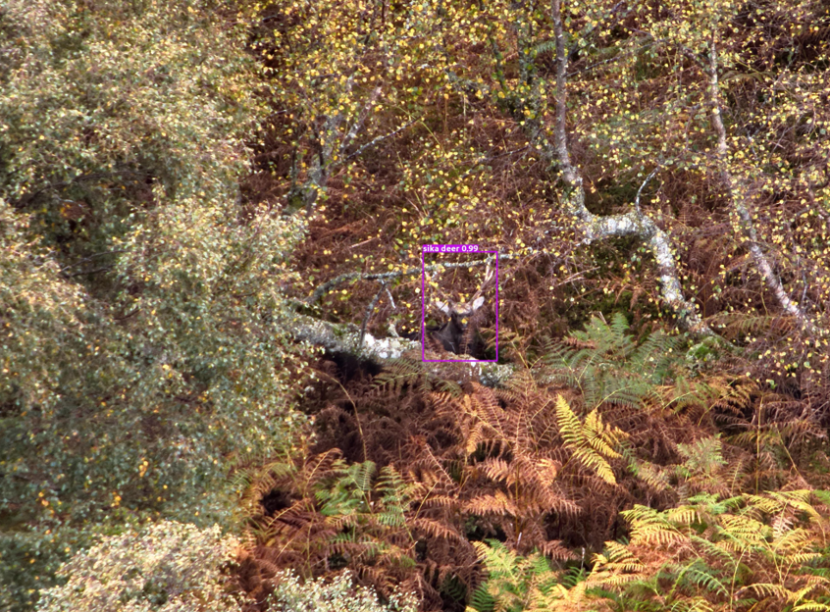
Sika deer in birch woodland
Click for a full description
This photograph is of a Sika deer in birch woodland with bracken in early autumn. The colours of the tree trunks and foliage make Sika deer very hard to locate and identify by eye. However, AI has identified the deer near the centre of the picture. Photograph courtesy of DroneWild.
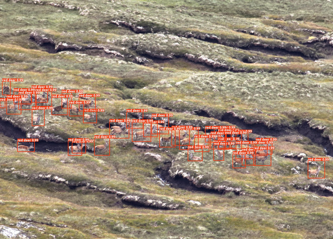
This is an oblique-angle aerial photograph of an upland hillside with a large group of red deer.
Click for a full description
AI has identified the individual deer enabling them to be counted accurately. Photograph courtesy of DroneWild.
Camera trapping provides a clear example of these approaches in practice. Large volumes of imagery can be generated over relatively short deployments, much of which may not contain animals. Web-based platforms such as Agouti are available to manage, classify and analyse these data, including automated species recognition and integration with analytical workflows. In a recent Glen Prosen trial for NatureScot, cameras were configured to capture images at regular intervals (e.g. every five minutes), resulting in hundreds of thousands of images. Automated workflows are then used to filter blank images and support species classification, substantially reducing the volume of data requiring manual review, although outputs still require human validation for reliable results.
In drone-based surveys, the best-practice approach described in this report is based on operator-led detection, where animals are identified during flight and imagery is collected accordingly. Automated detection is already under active development in support of this approach. For example, DroneWild are currently progressing AI-based image analysis within a Scottish Government and FLS funded project, and this work will be important in determining how automated processing can support larger survey coverage and improve consistency of interpretation. As these approaches develop, there is growing potential for detection to shift from the operator to AI-supported systems, including near real-time detection during surveys and more targeted image acquisition. Alternative approaches also exist, in which imagery is collected systematically across large areas and processed post hoc, but these are less aligned with the approach emphasised here.
Another development of the DroneWild project is automatic map production and density calculations by the model purely from reading the images and the meta data. This area is likely to grow significantly in the years to come with automation making handling large datasets and outputs much easier.
The use of AI and ML also has an associated carbon cost, primarily linked to model development and training rather than routine implementation. While this cost is likely to be small relative to wider survey operations, it should be recognised where large models or repeated training are required.
8.3 Scaling coverage: fixed-wing UAVs and aerial systems
The most significant near-term platform development is fixed-wing UAV technology. Compared to multirotor systems, fixed-wing UAVs offer substantially greater flight time and range and can cover large open landscapes rapidly. Faster coverage reduces the risk of deer moving between survey segments and may improve the practical feasibility of surveying very large areas within a short temporal window. Fixed-wing systems may also offer operational and carbon advantages relative to helicopters, depending on deployment scale.
Detection performance is not fundamentally different from multirotor UAVs: canopy structure and vegetation density remain limiting. Fixed-wing systems have historically lacked the ability to hover/interrogate a subject easily in woodland and were therefore best suited to open upland, non-leafed woodland, and structurally open habitats. However, this distinction is beginning to reduce as more manoeuvrable platforms emerge, capable of slower flight, tighter turning and short-duration loitering over areas of interest. In addition, the development of vertical take-off and landing (VTOL) systems means that fixed wing UAVs do not always now require dedicated space for take-off and landing, increasing their operational flexibility.
In comparison to quadcopters, costs are typically higher. Most importantly, their large-area potential depends on regulatory permission. Without Beyond Visual Line of Sight (BVLOS) approval under Civil Aviation Authority (CAA) regulations, operations may be restricted to Visual Line of Sight (VLOS), limiting their effective coverage advantage compared to quadcopters. Recent changes to the regulatory environment under the new SORA (Specific Operations Risk Assessment) system provide a clear pathway for BVLOS operations. However, approval is still required for specific operating conditions, including aircraft system, operating procedures and airspace environment and large-scale wildlife survey applications remain untested.
The combination of fixed-wing UAVs and AI-based image processing is particularly promising. Large areas can be surveyed efficiently, and automated processing can handle the increased data volume. As AI capabilities develop further, including near real-time, onboard detection and classification, there is increasing potential for systems that combine wide-area coverage with improved manoeuvrability and the ability to identify and respond to detections during flight. This pairing, along with the change in regulation, offers one of the clearest pathways for improving large-area abundance estimation in many landscapes, subject to regulatory and operational feasibility.
8.4 Satellite and existing aerial imagery
A different approach to expanding spatial coverage is to analyse high-resolution satellite or aerial imagery that has already been collected for mapping, land management, or commercial earth observation. Unlike the fixed wing or quadcopter drones systems, which rely on thermal sensors to detect animals during dedicated surveys, these approaches use very-high resolution optical imagery (RGB or multispectral). These datasets can be commissioned or may be available having been collected routinely for other purposes. This creates the possibility of retrospectively analysing animal distributions across large areas and potentially across multiple years. Because the satellites are already in place, or the imagery already exists, the additional operational or carbon cost for counting deer is likely to be lower.
Animals are identified within these images using artificial intelligence and machine-learning approaches that detect potential animals from their size, shape, contrast, and shadow patterns. Early trials undertaken for NatureScot examined both commercial satellite imagery (for example from platforms such as Maxar WorldView or Airbus Pleiades, typically providing spatial resolutions of around 30–50 cm) and existing aerial photography datasets (such as the UK Aerial Photography Great Britain (APGB) programme), which commonly provide finer resolutions of approximately 12–25 cm. By contrast, thermal satellite imagery has spatial resolutions of tens to hundreds of metres and is therefore far too coarse to detect individual animals.
Results indicated that higher-resolution aerial imagery performed better than satellite imagery, allowing individual red deer to be detected although only in favourable conditions in open upland landscapes, and it was not possible to age them. Detection success varied with image quality, seasonal vegetation cover, and atmospheric conditions, and was substantially reduced where dense vegetation limited visibility.
Since those trials were undertaken, the number of satellites capable of collecting very-high-resolution imagery has increased. New constellations such as Pleiades Neo and WorldView Legion provide additional platforms capable of ~30 cm imagery and substantially improved revisit frequency. These developments increase the availability of suitable imagery and may improve the potential for repeated observations or seasonal comparisons. At the same time, rapid improvements in artificial intelligence and machine learning methods for object detection may further improve the reliability of automated animal detection as larger training sets become available.
Similar satellite-based detection approaches have been demonstrated for other species, including elephants (Duporge e al 2021), migratory wildebeest (Duporge et al, 2025), and albatross (Fretwell et al, 2017). These applications generally involve large animals occurring in open landscapes and/or dense aggregations, conditions that are more favourable for detection than those found in many Scottish deer habitats. Continued improvements in imagery and automated detection may further increase capability in open environments, suggesting that these approaches may have greatest potential in open upland landscapes or as complementary tools at larger landscape scales. However, the fundamental requirement that animals must be visible from above means that dense vegetation will remain a constraint in many Scottish landscapes.
8.5 Sampling-based survey designs
For survey methods that aim to obtain a complete count of animals present at a given time, achieving full spatial coverage can become impractical in large or heterogeneous sites. This is especially relevant for aerial census approaches such as drone surveys, where surveying very large areas within a sufficiently short time window may be difficult. In such cases, structured sampling – using transects, systematic blocks, or stratified plot designs – provides a practical alternative. It reduces field effort while allowing density to be estimated for the surveyed area with explicit uncertainty. Trials undertaken for NatureScot using quadcopter drones indicate that such approaches are operationally feasible and may merit further evaluation where complete aerial coverage is impractical.
Sampling does not resolve the problem of habitats that are not surveyed or where detection is not possible (e.g., dense canopy or thicket). If a habitat component is effectively unobservable from the chosen platform, it remains an unsurveyed stratum under both census and sampling approaches. The benefit of a structured design is that it forces this issue to be explicit: surveyed and unsurveyed components are clearly defined, and uncertainty can be quantified for the surveyed area while unsurveyed habitat is addressed through complementary methods (e.g., camera, dung, genetic approaches), targeted calibration work, or clearly reported as an additional source of uncertainty rather than being implicitly treated as zero.
8.6 Genetic and DNA-based developments
Where visual detection is unreliable, advances in genetic analysis provide an extension of existing dung-based approaches. DNA-based capture–recapture enables identification of individuals from non-invasive samples (dung or hair) and estimation of abundance with explicit uncertainty (Lukacs & Burnham, 2005). This approach is particularly useful in habitats such as dense woodland where animals remain unavailable to direct observation.
Close-kin mark–recapture methods, which incorporate parent–offspring and half-sibling relationships, provide a further extension of these approaches (Babyn et al., 2024). These methods are likely to be most effective in higher-fecundity species such as roe deer, while their application is more limited in lower-fecundity species such as red deer and sika deer due to reduced detectability of kin pairs and therefore weaker statistical power.
Laboratory costs and sampling logistics and the limited availability of suitable UK laboratory capacity for routine high-throughput wildlife genotyping at scale currently constrain the wide-spread application of genetic methods. Thus, it is most suited to targeted application rather than routine large-scale deployment.
As a result, these approaches are unlikely to be cost-effective where the sole objective is to derive abundance estimates alone but are particularly valuable when applied to questions of population structure, dispersal, and connectivity, helping to identify landscape units that function as coherent populations and thereby informing the appropriate spatial scale for management. There may also be potential to explore genetic analysis using samples from culled deer.
8.7 Camera approaches to movement and exchange
Beyond their use for density estimation, camera-based approaches may provide insight into movement and exchange where identifiable corridors exist, for example in peri-urban landscapes or between open upland and adjacent woodland. In these contexts, cameras can help improve understanding of how animals redistribute between observable areas within and across sites, clarifying whether differences in counts reflect true demographic change or short-term movement.
Cameras may also provide information on movement between observable and unobservable habitats, such as dense woodland and deep canopy cover. In these cases, cameras, may help assess the extent to which deer move into and out of areas that are not surveyed.
The objective here, is not direct population estimation, but learning more about spatial redistribution and how this may influence interpretation of survey results. Methods for incorporating such movement or exchange information into population assessment need development.
8.8 Integration, modelling and monitoring design
As surveying expands across landscapes and scales, increasingly large and growing datasets on deer populations are becoming available from a range of sources. These include aerial surveys such as helicopter and drone counts, dung surveys, culling records, demographic information and citizen science data. Integrating these different sources offers considerable potential to estimate deer densities and trends at regional and national scales. However, doing so requires statistical approaches that can account for differing observation processes, spatial coverage, and potential biases in where surveys occur. In addition, some datasets are collected by, or for, private landowners and may be subject to confidentiality or data-sharing constraints, which can limit their availability for large-scale analyses.
At the scale of individual sites or management units, approaches such as data integration (Zipkin et al, 2021) and Integrated Population Models (Schaub & Abadi, 2011) provide one way of addressing these challenges. These approaches allow count data, time-integrated methods, and demographic information to be combined while explicitly separating state and observation processes. These approaches also provide an opportunity to identify which sources of information contribute most to reducing uncertainty and improving precision, helping to target future data collection more effectively.
At larger scales, approaches such as density surface modelling linking observed densities at survey sites to environmental covariates, allows prediction of abundance across unsurveyed areas (Bouchet et al, 2020). Environmental covariates may increasingly be derived from satellite or other remotely sensed imagery, including high-resolution habitat maps, vegetation indices, canopy structure proxies, and landscape fragmentation metrics. These approaches are essential at regional and national scales, where complete coverage is not achievable.
Improvements in inference are likely to depend not only on analytical integration of existing datasets but also on how future data are collected. Many existing datasets arise from surveys commissioned for individual estates or projects and may therefore be unevenly distributed across habitats, regions, or management systems. Structured monitoring programmes can help address these gaps by ensuring that surveys provide more representative coverage or by targeting additional surveys in areas where uncertainty is greatest. The importance of consistent survey design, spatial coverage, and repeatability for estimating trends in deer populations has been highlighted previously (Albon et al., 2019) and remains a key consideration for future monitoring. Adaptive schemes where survey designs can be refined over time as new information becomes available (Henrys et al 2024.,) may also provide useful.
In the longer term, the combination of repeated surveys, environmental data and integrated modelling frameworks may support more integrated monitoring systems, in which multiple data streams are brought together to provide updated assessments of deer populations. Such approaches could move towards more dynamic systems (sometimes referred to as “digital twins”), where new data are incorporated as they become available to progressively improve regional and national estimates of deer distribution and abundance and change over time.
For all of these approaches, the quality and structure of the underlying data are critical. In particular, consistent and well-documented metadata describing survey methods, spatial coverage, timing, and limitations are essential to enable datasets to be combined and interpreted correctly. Without this, differences between surveys may be difficult to disentangle from real changes in deer populations (Zipkin et al., 2021).
8.9 Emerging approaches
Acoustic monitoring (Enari et al, 2017) has potential in specific contexts, particularly during periods of high vocal activity such as the rut. Spatially explicit acoustic capture–recapture methods can, in principle, estimate density from calling individuals, but require strong assumptions about vocalisation rates and detection distances (Marques et al. 2013). Acoustic monitoring is therefore best viewed as a targeted tool for particular species or seasons rather than a general solution for abundance estimation.
8.10 Overall perspective
The most promising developments are not isolated technologies but combinations of approaches that address different components of the monitoring problem. Fixed-wing UAVs coupled with automated image analysis offer potential for efficient large-area surveys in open habitats. Analysis of high-resolution aerial or satellite imagery may also provide opportunities to detect animals or examine distribution patterns across large spatial areas with minimal additional carbon and operational cost, particularly in open landscapes. Sampling-based survey designs may provide a defensible alternative to attempting full coverage in heterogeneous landscapes.
Complementary methods remain important where direct detection is limited. Camera-, dung-, and genetic-based approaches may strengthen inference where aerial observation is constrained. At larger spatial scales, satellite-derived habitat data support stratification and spatial modelling, helping to relate observed densities to landscape structure and extrapolate beyond surveyed areas.
Progress is therefore likely to depend increasingly on analytical integration of these different data sources. Data fusion and Integrated Population Models and related approaches provide the analytical framework to combine these elements while explicitly quantifying uncertainty.
No development removes the ecological constraints of dense canopy or redistribution in open systems. Progress is therefore likely to come from targeted evaluation of these approaches under Scottish conditions, ideally where abundance is known, rather than from reliance on a single platform or method. The following chapter identifies priority areas for comparative testing and methodological development.
9. Design brief priorities for methodological development
These priorities identify areas where targeted testing and methodological development could most improve inference on deer abundance, trend, and management response across ecological contexts and spatial scales.
9.1 Woodland and dense canopy environments
Priority – clarify how different survey approaches perform and relate to one another in woodland environments where visibility varies.
- Conduct comparative trials of quadcopter drone, dung, camera (and where relevant vehicle-based) approaches in woodland, quantifying detectability and uncertainty across differing woodland structures, particularly dense canopy. Ideally where abundance is known.
- Analyse existing datasets from sites where dung and camera surveys have been undertaken to examine patterns of deer utilisation in dense canopy compared with more open areas.
- Assess how complementary survey approaches may be combined or cross-calibrated to improve inference where no single method provides adequate coverage.
- Link with ongoing NatureScot work on camera-based approaches in woodland.
9.2 Open upland and open landscapes
Priority – improve spatial coverage and operational efficiency in landscapes where aerial detection is feasible.
- Evaluate improvements in helicopter-based surveys through the deployment of thermal imaging systems, particularly in comparison with existing visual surveys.
- Undertake trials of fixed-wing UAV systems to determine their potential for extending survey coverage across large upland areas where quadcopter deployment becomes operationally demanding.
- Evaluate sampling-based survey designs where full aerial coverage within a survey window is not achievable.
- Evaluate the potential role of automated detection and classification of deer from aerial imagery using machine-learning approaches to improve processing efficiency and consistency.
- Re-examine the potential for retrospective or prospective analysis of high-resolution satellite or aerial imagery to examine deer distributions across large open landscapes.
- Compare operational performance, detection, carbon implications and cost-efficiency across helicopter, quadcopter, fixed-wing UAV and retrospective imagery approaches, potentially using comparative field trials.
9.3 Camera approaches for movement and corridor processes
Priority – understand movement influencing interpretation of surveys.
- Pilot camera-based approaches to examine movement and exchange along identifiable corridors (e.g. peri-urban green corridors, upland–woodland transitions).
- Assess feasibility of boundary-based monitoring approaches, particularly at interfaces between observable habitats (such as open hill) and unobservable habitats (such as dense canopy).
- Evaluate how movement information may support interpretation of survey results.
9.4 Integration and scaling
Priority – strengthen inference across habitats and spatial scales through coordinated data collection, integration and monitoring design.
- Develop modelling frameworks capable of integrating multiple survey types (e.g. helicopter, drone, dung, camera) with culling records and demographic information, to support inference at the landscape scale, and combine these with spatial environmental data to enable extrapolation beyond surveyed areas and across regional and national scales.
- Examine the range of existing datasets across Scotland, and identify barriers to their integration including data accessibility, consistency and confidentiality constraints.
- Explore methods for identifying appropriate landscape-scale monitoring units in different ecological contexts, recognising that the spatial scale of deer populations may vary with species behaviour, habitat configuration and movement patterns.
- Explore how coordinated monitoring programmes across sites and regions could improve representativeness of surveys and allow new data to progressively improve regional and national population estimates
9.5 Overall priorities
- Highest immediate priority – improving interpretation of deer abundance and site use in woodland and dense canopy environments where visibility limits detection
- Strategic priority – cataloguing existing survey datasets and developing analytical frameworks for their integration, developing coordinated survey and monitoring approaches capable of supporting landscape, regional and national population assessment,
- Operational development priority – improving survey coverage and efficiency in large open landscapes, including evaluation of: fixed-wing UAV systems; improvements in aerial detection technologies; and approaches that reduce operational and carbon costs
- Supporting developments – sampling design, understanding deer movement, and combining survey methods for heterogeneous landscapes.
References
Albon, S.D., Irvine, R.J., Halvorsen, O., Langvatn, R., Loe, L.E., Ropstad, E., Veiberg, V. and Stien, A. (2019) Updating the estimates of national trends and regional differences in red deer densities on open-hill ground in Scotland. Scottish Natural Heritage Research Report No. 1149.
Boer-Cueva, M., Bombieri, G., Centomo, E., Salvatori, M., et al. (2026) Hunting and outdoor recreation affect large herbivore activity patterns more than natural predators in a human-dominated landscape. Ecology and Evolution. Available online: 16 February 2026.
Bouchet, P.J., Miller, D.L., Roberts, J.J., Mannocci, L., Harris, C.M. and Thomas, L. (2020) dsmextra: extrapolation assessment tools for density surface models. Methods in Ecology and Evolution, 11, pp.1464–1469.
Buckland, S.T., Rexstad, E.A., Marques, T.A. and Oedekoven, C.S. (2015) Distance sampling: methods and applications. Cham: Springer.
Campbell, D., Swanson, G.M. and Sales, J. (2004) Comparing the precision and cost-effectiveness of faecal pellet group count methods. Journal of Applied Ecology, 41(6), pp.1185–1196.
Daniels, M.J. (2006) Estimating red deer abundance: comparison of methods. Journal of Applied Ecology, 43(2), pp.223–231.
Duporge, I., Isupova, O., Reece, S., Macdonald, D.W. and Wang, T. (2021) Using very-high-resolution satellite imagery and deep learning to detect and count African elephants in heterogeneous landscapes. Remote Sensing in Ecology and Conservation, 7, pp.369–381.
Duporge, I., Wu, Z., Xu, Z., Gong, P., Rubenstein, D., Macdonald, D.W., Sinclair, A.R.E., Levin, S., Lee, S.J. and Wang, T. (2025) AI-based satellite survey offers independent assessment of migratory wildebeest numbers in the Serengeti. PNAS Nexus, 4(9).
Eggers, J., Maroschek, M., Seidl, R., Greiner, S., Loretto, M., Seiboldm S,m Reiner, R. (2025) Navigating a landscape of contrasting hunting regimes and habitats: red deer responses to risk and resources. Wildlife Biology
Enari, H., Ouda, K., Yoshita, M., Juno, T. and Ojuda, K. (2017) Feasibility assessment of active and passive acoustic monitoring of sika deer populations. Ecological Indicators, 79, pp.155–162.
Fretwell, P.T., Scofield, P. and Phillips, R.A. (2017) Using super-high resolution satellite imagery to census threatened albatrosses. Ibis, 159, pp.481–490.
Gilbert, N.A., Clare, J.D.J., Stenglein, J.L. and Zuckerberg, B. (2021) Abundance estimation of unmarked animals based on camera-trap data. Conservation Biology, 35(1), pp.88–100.
Henrys, P.A., Jarvis, S.G., Smart, S.M., Wood, C.M. et al. (2024) Adaptive sampling in ecology: key challenges and future opportunities. Methods in Ecology and Evolution.
LaRue, M.A., Salas, L., Nur, N., Ainley, D., Stammerjohn, S., Pennycook, J., Dozier, M., Saints, J., Stamatiou, K., Barrington, L. and Rotella, J. (2021) Insights from the first global population estimate of Weddell seals in Antarctica. Science Advances, 7(39).
Lukacs, P.M. and Burnham, K.P. (2005) Review of capture–recapture methods applicable to noninvasive genetic sampling. Molecular Ecology, 14(13), pp.3909–3919.
Marcon, A., Battocchio, D., Apollonio, M. and Grignolio, S. (2019) Assessing precision and requirements of three methods to estimate roe deer density. PLOS ONE, 14(10), e0222349.
Marques, T.A., Buckland, S.T., Bispo, R. and Howland, B. (2013) Accounting for animal density gradients using independent information in distance sampling surveys. Statistical Methods and Applications, 22, pp.67–80.
Marques, T.A., Thomas, L., Martin, S.W., Mellinger, D.K., Ward, J.A., Moretti, D.J. et al. (2013) Estimating animal population density using passive acoustics. Biological Reviews, 88, pp.287–309.
McMahon, T.A., Michel, N.L., Curry, C.M., Sikes, R.S. and Kolbe, J.J. (2021) Comparing unmanned aerial systems with conventional methodology for surveying a wild white-tailed deer population. Wildlife Research, 49(1), pp.1–12.
NatureScot (2008a) Best practice guidance: population assessment – open range counting (1)
NatureScot (2008b) Best practice guidance: population assessment – open range counting (2)
NatureScot (2025) Deer counts – deer groups: locations and group sizes from helicopter and ground-based counting operations.
NatureScot (2026a) Best practice guides: use of drones (UAVs) 1.
NatureScot (2026b) Best practice guides: use of drones (UAVs) 2.
NatureScot (no date) Deer management methods.
Newman, K.B., Buckland, S.T., Morgan, B.J.T., King, R., Borchers, D.L., Cole, D.J., Besbeas, P., Gimenez, O. and Thomas, L. (2014) Modelling population dynamics: model formulation, fitting and assessment using state-space models. Springer.
Paulsen, K.M., et al. (2023) How many reindeer? UAV surveys as an alternative to helicopter or ground survey methods for estimating population abundance in open landscapes. Remote Sensing, 15(9).
Pfeffer, S.E., Spitzer, R., Allen, A.M., Hofmeester, T.R., Ericsson, G., Widemo, F., Singh, N.J. and Cromsigt, J.P.G.M. (2018) Pictures or pellets? Comparing camera trapping and dung counts as methods for estimating population densities of ungulates. Remote Sensing in Ecology and Conservation, 4(2), pp.173–183.
Rowcliffe, J.M., Field, J., Turvey, S.T. and Carbone, C. (2008) Estimating animal density using camera traps without the need for individual recognition. Journal of Applied Ecology, 45(4), pp.1228–1236.
Schaub, M. and Abadi, F. (2011) Integrated population models: a novel framework for population analysis. Journal of Ornithology, 152(Suppl 1), pp.227–237.
Strath Caulaidh (2021) A strategic overview of wild deer population dynamics in the Cairngorms National Park. Report to the Cairngorms National Park Authority.
Swanson, G., Campbell, D. and Armstrong, H. (2008) Estimating deer abundance in woodlands: the combination plot technique. Forestry Commission Bulletin 128.
Wäber, K., Spencer, J., Dolman, P.M. (2013) Achieving landscape-scale deer management for biodiversity conservation: the need to consider sources and sinks. The Journal of Wildlife Management, 77(4), pp. 726–736
Zipkin, E.F., Zylstra, E.R., Wright, A.D., Saunders, S.P., Finley, A.O. and Dietze, M.C. (2021) Addressing data integration challenges to link ecological processes across scales. Frontiers in Ecology and the Environment, 19, pp.30–38.
Annex 1 – Site scenarios
Strathconon: Open Hill / Upland Systems
Strathconon is a large open upland system in the central Scottish Highlands (c. 37,600 ha) dominated by hill, moorland, blanket bog, and montane habitats. Vegetation is generally low and visibility is high, although bracken may locally reduce openness during summer. The estate spans valley floors to high-altitude ground and at this scale, it provides a coherent unit for interpreting population status and change.
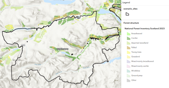
Figure A1. Map of Strathconon Estate with site boundary at time of drone survey (black line) and National Forest Inventory Scotland habitat classification.
Click for a full description
The classification categories are: Broadleaved; Conifer; Assumed woodland; Felled; Young trees; Grassland; Mixed mainly broadleaved; Mixed mainly conifer; Windblown; Ground prep; Other.
As in other large open upland systems, red deer in Strathconon show strong seasonal and social structuring. Hinds are often loosely “hefted” within broad ranges, while stags move more widely, particularly during the rut. Seasonal redistribution between high and lower ground is common and strongly influenced by weather and forage availability, altering where deer are located more than total population size at the landscape scale.
Within Strathconon, movement in and out of the estate is partly constrained in the north by railway lines and public roads, and elsewhere by water bodies and terrain. Although movement across some other boundaries occurs, particularly where adjacent habitats differ, the large spatial scale and social organisation mean that the core population behaves approximately as closed over short time periods.
Roe and sika deer are present locally, typically associated with patches of woodland or sheltered habitat. Their movement operates at a smaller spatial scale than red deer and their contribution to overall abundance is limited, though they may influence local variability within parts of the estate.
Because of the size of the site, the red deer population total is relatively stable over short time periods, although its distribution within the estate may vary greatly. This redistribution is driven by weather and forage, wider-ranging movement of stags relative to hinds, and limited movement across some boundaries.
As a result, changes in total numbers are driven mainly by demographic processes rather than movement from and to surrounding areas. This means that longer-term trends and responses to management are more likely to be detectable, especially when populations are compared at similar times of year and across the whole site to encompass seasonal movement.
Torrachilty: Commercial Upland Forestry
Torrachilty is a commercial upland forestry system characterised by a structurally complex mosaic of conifer plantation, mixed woodland, and open areas embedded within a wider open hill landscape. Dense canopy, varied topography, and clearfell cycles create strong spatial heterogeneity, with areas of high and low deer use occurring within the same site. Management, including night shooting and out-of-season culling occurs for all three species.
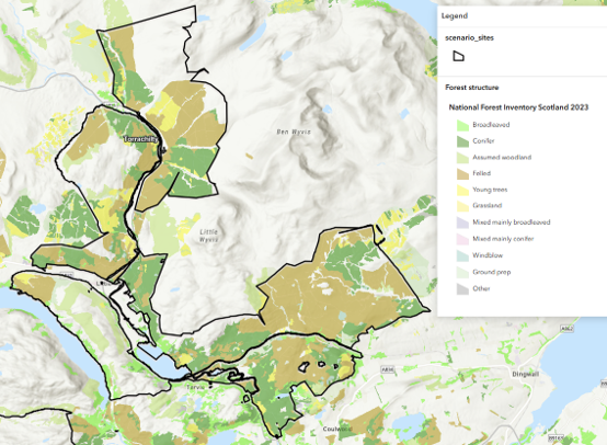
Figure A2 Map of FLS Torrachilty with site boundary (black line) and National Forest Inventory Scotland habitat classification.
Click for a full description
The classification categories are: Broadleaved; Conifer; Assumed woodland; Felled; Young trees; Grassland; Mixed mainly broadleaved; Mixed mainly conifer; Windblown; Ground prep; Other.
As in similar upland forestry systems, red deer using the site may behave in two ways: historic records show persistent red deer presence on the open hill around Torrachilty. These deer move into the woodland site mainly during poor weather or winter. Other red deer may remain within woodland throughout the year. Population numbers of red deer on the site are therefore strongly influenced by weather, forage, and disturbance.
Roe and sika show more localised spatial behaviour. Roe deer occupy relatively small, overlapping home ranges largely within woodland, while sika are closely associated with dense forestry, show limited seasonal movement, and are often more nocturnal.
As a result, the deer population within Torrachilty behaves as an open system, particularly for red deer. The main sources of state variability are immigration and emigration of red deer due to seasonality, weather and response to culling. For roe and sika, variability is more localised and reflects habitat structure and management within the woodland. In contrast to large open upland systems such as Strathconon, variation in population numbers at Torrachilty on a daily basis is likely higher in the short term and more often reflects movement rather than demographic change, making detection of trends and management effects more difficult at the site scale
Devilla - Lowland Commercial Woodland
Devilla Forest is a lowland mixed woodland system (c. 700 ha) comprising predominantly commercial Scots pine plantation interspersed with deciduous woodland along paths and edges of four lochs. It is mainly surrounded by woodland.
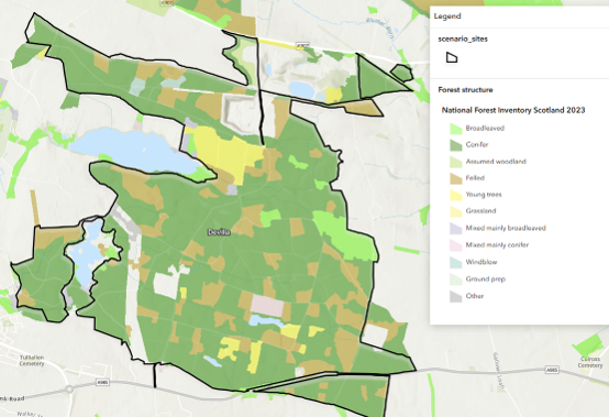
Figure A3 Map of FLS Devilla with site boundary (black line) and National Forest Inventory Scotland habitat classification.
Click for a full description
The classification categories are: Broadleaved; Conifer; Assumed woodland; Felled; Young trees; Grassland; Mixed mainly broadleaved; Mixed mainly conifer; Windblown; Ground prep; Other.
Roe deer dominate the system and largely determine state variability. They occupy relatively small, stable home ranges and tend to remain within the woodland for much of the time, particularly using dense cover during poor weather. Regular daily movements occur between woodland and surrounding farmland, especially at dawn, dusk, and overnight when deer move out to feed. Seasonal behavioural changes, particularly in spring when females expel yearlings and males re-establish territories, can temporarily increase movement and redistribution, though overall spatial stability remains relatively high compared with more mobile red deer systems. Sika and occasional red deer are present in smaller numbers.
Culling of roe and sika is carried out within Devilla and also occurs on surrounding farmland and neighbouring estates. The wider pattern of control is not fully known, but immigration is likely and the site may function partly as a sink where suitable habitat and local removals draw in deer from surrounding areas. Redistribution within the woodland and movement across its boundaries therefore influence local abundance alongside demographic change.
At the scale of Devilla, the roe deer population total is relatively variable within a day but stable between days, compared with commercial upland forestry, but is not fully closed. The main sources of state variability arise from local movement between woodland and farmland (within day variability), seasonal territorial behaviour and immigration leading to redistribution linked to management in Devilla and the surrounding area. Short-term variation in population totals and distribution may therefore reflect both local movement and demographic change. Longer-term trends and responses to management are generally more detectable than in highly open systems with herding species if populations are compared at similar times of the day (to remove within day variability) and times of the year (to remove seasonal variability).
Craigellachie - Semi-Natural / Native Woodland – Small, Highly Connected Systems
Craigellachie NNR lies on the eastern slopes of the Monadhliath range within the Cairngorms National Park and comprises a relatively small but structurally complex landscape ranging from approximately 225 to 535 metres in elevation. The site is example of a semi-natural woodland, in this case dominated by birch with roughly half of the area consisting of upland habitat. It sits within a wider mixed landscape of open hill, forestry, and more modified lowland habitats, and functions as part of a broader ecological system rather than as an isolated unit.
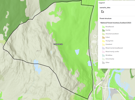
Figure A4 Map of Craigellachie with site boundary (black line) and National Forest Inventory Scotland habitat classification.
Click for a full description
The classification categories are: Broadleaved; Conifer; Assumed woodland; Felled; Young trees; Grassland; Mixed mainly broadleaved; Mixed mainly conifer; Windblown; Ground prep; Other.
Red and roe deer occur on the site, but their relationship to the area differs. Red deer use Craigellachie intermittently, primarily for shelter, forage, or seasonal movement between surrounding upland areas, and the site is best understood as one component of a larger population system rather than holding a discrete local population. Roe deer are more locally resident, occupying relatively small home ranges within the woodland, though they remain connected to neighbouring habitats and may move beyond the site. As a result, red deer presence can vary substantially over short periods, while roe deer tend to show greater local stability.
Management within Craigellachie is generally low intensity, with limited culling aimed at maintaining sustainable deer levels. However, surrounding landscapes are likely to exert a stronger influence on local dynamics. Movement from adjacent open hill and forestry may replenish deer removed within the site, and changes in management beyond the reserve may alter local abundance and distribution.
At the scale of Craigellachie, the deer population is not closed. Population totals of red deer will vary hugely reflecting the site as representing only part of their range providing the main source of state variability. Consequently, local population totals may fluctuate independently of underlying demographic change, making longer-term trends and responses to management difficult to detect at the site scale, especially for red deer, while roe deer may show relatively greater local stability.
Agricultural Landscapes – Highly Connected, Open Systems
This agricultural landscape represents a typical lowland arable–pastoral system in northeastern Scotland, dominated by open farmland interspersed with hedgerows, small woodland fragments, field margins, and rough grassland. These features provide shelter, movement corridors, and seasonal forage within an otherwise open and highly connected landscape. Surrounding areas are generally similar in character, with few barriers to deer movement.
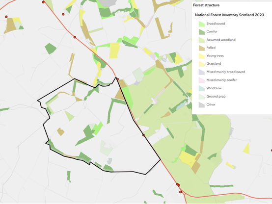
Figure A5 Map of an arable site with site boundary (black line) and National Forest Inventory Scotland habitat classification, major road (red line) and deer vehicle collisions (red dots).
Click for a full description
The classification categories are: Broadleaved; Conifer; Assumed woodland; Felled; Young trees; Grassland; Mixed mainly broadleaved; Mixed mainly conifer; Windblown; Ground prep; Other.
Roe deer typically dominate in such systems and largely determine population behaviour. They occupy relatively small home ranges but, in large open agricultural settings, may use hedgerows, ditches, and field margins for cover rather than remaining within woodland. Daily movement between sheltered cover and feeding areas is common, with deer often more active in open fields at dawn, dusk, and during the night. Seasonal changes in crop availability, disturbance, and vegetation structure influence where deer concentrate. Other species such as red, sika, or fallow may occur locally and may use farmland opportunistically, particularly when crops provide forage, but they generally contribute less to overall abundance.
Direct management within a single agricultural holding may be limited, and the surrounding landscape often exerts a stronger influence on local dynamics. Because habitat is continuous and highly connected, deer frequently move between neighbouring farms and, where available, woodland patches. Local removals may therefore be offset by immigration, while management elsewhere may influence numbers within the site.
At the scale of an individual agricultural area, the roe deer population total may vary (like Devilla) within a day due to regular movement between cover and feeding areas but can appear relatively stable from day to day, and the population is not fully closed. At certain times of year, however, wider movement of additional deer in response to crop availability, disturbance, or seasonal behaviour can alter local numbers substantially. The main sources of state variability therefore arise from daily feeding movements, seasonal redistribution linked to crops and habitat use, and movement into and out of the surrounding landscape. Short-term variation in population and distribution may reflect both local stability and periodic movement, and defining a fixed local population can be difficult as numbers may change over the course of the year. Longer-term trends and responses to management are therefore most detectable when populations are compared at similar times of day and season and, where possible, at spatial scales large enough to encompass wider movement.
Easterhouse - Peri-Urban Landscapes – Fragmented, Behaviourally Modified Systems
This peri-urban landscape comprises a mixture of housing, transport infrastructure, greenspace, woodland patches, and informal open ground. Roe deer dominate and often occur at relatively high densities, typically occupying small home ranges and showing strong habituation to human presence. Woodland fragments and greenspace provide cover and resting areas, while open grassland and edge habitats provide feeding opportunities.
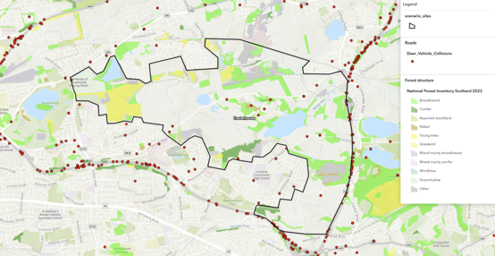
Figure A6 Map of Easterhouse with site boundary (black line), National Forest Inventory Scotland habitat classification and deer vehicle collisions (red dots).
Click for a full description
The majority of the red dots where deer vehicle collisions have occurred are on major roads. The classification categories are: Broadleaved; Conifer; Assumed woodland; Felled; Young trees; Grassland; Mixed mainly broadleaved; Mixed mainly conifer; Windblown; Ground prep; Other.
Movement within the site is partly constrained by motorways, railway lines, and dense urban development, which create locally semi-contained populations. Despite this, redistribution still occurs within the available habitat, and some movement takes place along green corridors or less fragmented edges of the landscape. Roe deer frequently show strong short-term site fidelity, though individuals may shift location following disturbance, territorial pressure, or mortality events such as vehicle collisions.
Direct culling within urban woodland areas is often limited or absent, although deer-vehicle collisions and occasional management on surrounding farmland or private land may influence local population structure. Where removals occur nearby, local redistribution or limited immigration may follow, depending on the availability of connected habitat. Human disturbance, fragmentation, and mortality therefore play major role in shaping spatial distribution and local population dynamics.
At the scale of a peri-urban site, the roe deer population total is relatively stable over short periods due to restricted movement and small home ranges, but the population is not fully closed. The main sources of state variability arise from local redistribution within fragmented habitat, occasional movement along connected corridors, displacement following disturbance or mortality, and redistribution linked to management in surrounding areas. Short-term variation in population totals and distribution therefore often reflects local movement and behavioural response rather than demographic change. Longer-term trends and responses to management may be detectable at the local scale, but interpretation depends on consistent spatial extent and an understanding of connectivity to surrounding populations, which can influence whether local numbers reflect a semi-contained population or part of a wider urban system.