NatureScot Research Report 1305 - Mapping prey resources of wintering seaducks within two marine Special Protection Areas in Scotland
Year of publication: 2026
Authors: Tillin, H.M., Holt, B., Grundy, S. Lear, D.
Cite as: Tillin, H.M., Holt, B., Grundy, S. Lear, D. Mapping prey resources of wintering seaducks within two marine Special Protection Areas in Scotland. NatureScot Research Report 1305.
Keywords
Seaduck; marine habitat; biotope; predictive modelling; predictive mapping; Marine Protected Areas; foraging; prey resources; Moray Firth Special Protection Area; Outer Firth of Forth and St Andrews Bay Complex Special Protection Area
Background
A number of Special Protection Areas (SPAs) in Scottish inshore marine waters have been designated to safeguard notable populations of seabirds and inshore wintering waterfowl (divers, grebes and seaducks). These waterfowl feed upon a range of prey, many of which live in or on the seabed and in some instances form biogenic (living) habitat features. The importance of prey-supporting habitats to the relevant bird populations and to the overall integrity of these marine protected areas is recognised in the sites’ Conservation Objectives. These objectives include the maintenance or, where appropriate, restoration of the supporting habitats and processes relevant to qualifying bird features and their prey resources.
The overarching aim of this project was to evaluate the potential for predictive modelling and mapping of the extent of important seaduck prey resources within two such marine protected areas. The specific objectives were to generate georeferenced datasets of known and predicted distributions and extents of principal bivalve and gastropod prey resources and associated supporting seabed habitats/ biotopes for five species of seaduck found within the Outer Firth of Forth and St Andrews Bay Complex (OFFSABC) SPA and the Moray Firth SPA. The project was desk-based and used existing information on environmental variables and survey data relating to the relevant prey species and associated benthic habitats.
Approach
The project initially considered 16 bivalve or gastropod species identified in previous scoping work as forming an important part of the winter diets of the five seaduck species. This list was reduced following removal of Pharus legumen, which is not considered to be readily available as prey, and three non-native species for which insufficient data were available to predict and map distributions. The project focused primarily on the 12 remaining native prey species and included initial evidence reviews for each. An evidence review was also completed for the invasive species Ensis leei, which has been associated with trophic disruption elsewhere in Europe.
The project then trialled two approaches to predict and map suitable habitats for the 12 native prey species within the target SPAs:
- mapping of predicted prey species distributions based on Generalised Additive Models (GAM); and,
- mapping of biotopes associated with these prey species.
The species modelling approach examined associations between the occurrence and abundance of target prey taxa and underlying environmental variables to inform predictive mapping of these taxa in the target sites. The second approach used documented associations between prey taxa and biotopes within the UK Marine Habitat Classification to enable prediction of prey occurrence and abundance within previously mapped benthic habitats. The evidence reviews for each prey species provided additional information to assess habitat suitability and to evaluate the results of the two approaches.
This report should be read with reference to the associated Supplementary Technical Report (STR), which includes all the mapped outputs and the species evidence review results along with information on underlying data
Main findings
- The project has shown the value of predictive species modelling and biotope analysis and mapping approaches to support identification of suitable habitats for seaduck prey within large marine SPAs. However, outputs should be interpreted carefully alongside information on the ecology of prey species and observed seaduck habitat preferences and taking into consideration the evaluated model performance for predicting presence and absence.
- Both approaches discriminated between areas of suitable and unsuitable prey-supporting habitats within the target SPAs and also illustrated variation in likelihood of occurrence.
- However, there were notable differences in the predicted prey presence and abundance/biomass maps between the outputs based on species models and those based on biotope analysis.
- These different approaches allowed evaluation of the outputs in the context of the prey species evidence reviews. Mapped outputs were considered to accord with suitable habitats in many instances, although exceptions have been described.
- For three species of seaduck, combined principal prey species maps were also evaluated against known distribution of these birds in both SPAs. This found that the mapped outputs generally predict high principal prey biomass in areas with greater numbers of seaduck.
- Ground-truthing would be needed for full evaluation of the results.
- Available evidence varies considerably between species; larger and commercially exploited species, such as Cerastoderma edule, Mytilus edulis and Mya arenaria, were the subject of more habitat studies. Little information was available for smaller species that were not of conservation or economic importance such as the gastropods, Lacuna vincta, Margarites helicinus and Hydrobia spp.
- There was similar variation in numbers of surveys that could be used to support predictive species model development and testing. For one species there was no survey data from within the SPAs and for half the species there were no abundance records from within the SPAs.
- There was a large degree of overlap between species presence and absence across assessed environmental gradients (for temperature, salinity, wave energy, substratum and depth) with little evidence for specific habitat requirements for many of the assessed species. Environmental variables typically have low discriminatory value in determining areas where species may occur from those where they are absent.
- In addition, many factors that are important to benthic species, and that influence distribution, cannot be easily incorporated into models, especially where these represent variables that are not readily measured (e.g. food resources or environmental factors that are temporary, such as episodes of low or high salinity, oxygen depletion or even wind-driven dispersal events).
- Overall, optimal species model performances were not strong. Confidence in mapped outputs based on likelihood of prey species occurrence was also typically low or very low. However, for species with more specific habitat requirements such as Donax vittatus and Astarte elliptica, abundance models with greater predictive power could be developed than for those, such as Mytilus edulis and Spisula subtruncata, which have broader habitat tolerances.
- Prey size is a key parameter determining prey suitability for seaduck and the survey data did not record lengths for species such as M. edulis and Mya arenaria which may reach a size whether they are no longer predated upon by seaduck.
- The UK Marine Habitat Classification supporting records form the basis of the biotope associations used to underpin the biotope mapping. This classification is a tool to describe and manage marine habitats and does not include all the species that may be found in a recognisable biotope or habitat. The number of records and the fidelity of species to biotopes also varies considerably and caution should be exercised in interpreting associations and outputs. . Species may be absent from habitats in which they are considered to be characterising and conversely may be present in other habitats where they are not characteristic.
- The limitations to both approaches are further detailed and discussed in the report.
- The Excel spreadsheet developed for the biotope analysis, based on the UK Marine Habitat Classification structure, can in future be updated with additional prey species and can support evaluation of likely prey species distribution and availability for other areas with habitat maps that can be related to the classification.
Acknowledgements
The MBA project team would like to thank the NatureScot project team, data suppliers and a number of other people who provided advice and help. The NatureScot team’s inputs are appreciated by the MBA project team and we are grateful to have had their support and expert advice throughout. Kate Thompson as project manager provided invaluable oversight and was entirely supportive throughout the project and review process. Rona Sinclair provided access to data and advice on sourcing further data as well as valuable input to project tasks and support for the integration of the GIS outputs to NatureScot’s systems. Ben James provided information on methodology, habitat mapping and additional comments that improved the final reports. Access to Oceanwise Marine Themes Digital Elevation Model (DEM) data was facilitated by the NatureScot Technology and Digital Service Team.
Colleagues at the University of Plymouth (Tom Mullier, Matt Ashley) and AVS Developments Ltd (Steve Pegg) freely contributed advice on previous versions of ArcMap and their assistance is gratefully acknowledged.
Contents
- Keywords
- Background
- Approach
- Main findings
- Acknowledgements
- Introduction
- Project background – preceding studies
-
Methodology
- Mapping seaduck prey within SPAs using predictive modelling
- Task 1: Evidence review
- Task 2: Data collation
- Task 3A: Data Preparation
- Task 3B: Model building
- Task 3C: Prediction, testing and mapping
- Mapping seaduck prey within SPAs using predictions based on biotope analysis
- Task 4A Evidence review: principal prey species occurrence and abundance within biotopes
- Task 4B Estimating prey abundance and occurrence probability within UKSeaMap polygons.
- Task 4C Mapping and confidence assessments (likelihood of presence)
- Review of outputs
-
Results
- Species modelling: evidence review and data availability
- Species modelling: model characteristics and performance
- Biotope analysis
- Overview of outputs for prey species
- Astarte elliptica
- Cerastoderma edule
- Cerastoderma glaucum
- Donax vittatus
- Hydrobia spp.
- Lacuna vincta
- Limecola balthica
- Macoma spp.
- Margarites helicinus
- Mya arenaria
- Mytilus edulis
- Spisula subtruncata
- Seaduck prey maps
- Common eider
- Long-tailed duck
- Common scoter
- Discussion
- Conclusions and Recommendations
Introduction
Scotland’s marine environment is recognised as an area of outstanding importance for a number of European bird species, which use these productive temperate waters in the winter period as an area to moult, roost and feed.
The Birds Directive (EC Directive on the conservation of wild birds consolidated in 2009 as 2009/147/EC2, replacing the original 1979 Directive), requires Member States to establish a national network of Special Protection Areas (SPAs) on land and at sea. This is one of several conservation measures that contribute to the protection of rare, vulnerable and migratory bird species and has been a major driver of UK bird conservation action over the past three decades. In the terrestrial environment, the Scottish SPA network includes breeding seabird colony SPAs and estuarine SPAs for some seaduck and grebe species.
A more recent focus on the marine environment (Marine SPA selection process) has included classification of 14 marine SPAs in Scotland for the protection of seabirds, divers, grebes and seaduck. Nine of these sites include one or more species of inshore wintering waterfowl (divers, grebes, seaduck) as qualifying features. Marine Protected Areas, including SPAs, contribute towards achieving Favourable Conservation Status of vulnerable species and habitats across the Atlantic Biogeographic Region.
These inshore wintering waterfowl feed upon a range of prey, many of which live in or on the seabed and in some instance form biogenic (living) habitat features. The importance of these prey resources and associated supporting habitats to the relevant bird populations and the maintenance of the integrity of these marine protected areas is recognised in the SPA Conservation Objectives. These objectives include the maintenance or, where appropriate, restoration of the supporting habitats and processes relevant to qualifying bird features and their prey resources.
Meeting these objectives requires appropriate management of human activities within these sites, including robust evidence-based assessments of potential impacts of proposed developments on prey resources and their supporting habitats.
The marine SPAs are multi-species sites within which the distributions of individual bird species reflect different prey preferences and foraging behaviours. This means that particular areas of specific habitats within a much larger site may potentially be of critical importance to one or more of the qualifying bird features and hence to the maintenance of overall site integrity. Effective site management to meet the Conservation Objectives therefore requires an understanding of the distribution and extent of relevant prey and associated supporting habitats within individual SPAs.
Due to the relative inaccessibility of subtidal habitats, compared with intertidal and terrestrial habitats, mapping the distribution of prey species over large areas is challenging. Typically diver or boat based surveys are required. In addition, some of the prey species are infauna living within the surface layers of sediment. Sampling these requires intrusive survey techniques while processing sediment samples is time consuming and requires taxonomic expertise.
These limitations mean that only small areas of large marine sites can be mapped directly using data surveys and sampling. However, approaches that can use readily collected and accessible data to predict suitable habitat presence and extent for prey species could be used to support cost-effective site management.
Project background – preceding studies
Identification of principal prey taxa
The work reported on here builds upon two previous studies commissioned by NatureScot to explore potential for mapping prey resources of inshore wintering waterfowl. An (unpublished) literature review of the marine diets and foraging behaviours of the wintering waterfowl species included as qualifying features in Scottish marine SPAs was commissioned by NatureScot and completed by the British Trust for Ornithology (BTO) in March 2018 (Woodward and Humphreys, unpublished).
The focus of the literature review was on eleven inshore wintering waterfowl species, including the five seaduck species (common eider, long-tailed duck, common scoter, velvet scoter and greater scaup) that were the focus of the current study. The outputs consist of a methodology report and a high level summary of findings and Excel spreadsheets detailing the literature review findings. The project provided a comprehensive review of diet and foraging behaviour and ecology, including dive depths.
This review was followed by a scoping study, undertaken by Envision Ltd, in 2018/2019 (Sotheran et al., unpublished). Based on the BTO literature review and some additional literature, the scoping project determined the dietary importance of various prey, either as named species (Mytilus edulis) or as prey categories (e.g., ‘bivalves’, ‘amphipods’), for each bird species. Prey were assessed as “principal prey taxa” if any primary or secondary literature source from Scotland, UK and Ireland or Europe identified the prey as Main or Important (i.e. forming 50% or more of diet) and the assessment was supported by multiple sources.
Bivalves were identified as a principal prey resource for the five seaduck species (common scoter, velvet scoter, common eider, long-tailed duck and greater scaup) considered in the literature review. M. edulis was identified as a principal prey resource for all but velvet scoter, for which it is of lesser importance. The largest number of bivalve taxa identified as principal prey were for common scoter. Of those birds feeding extensively on bivalves, the most varied diet is for long-tailed duck, with gastropods, crustacea and fish also identified as principal prey resources. Crustacea are an additional principal prey resource for common eider and have also been recorded in the diets of common scoter and several fish-eating species.
Of the remaining six species considered in the BTO review, common goldeneye wintering in marine areas were identified as feeding principally on gastropods and crustacea, with bivalves, including M. edulis, and other invertebrates identified as of lesser importance. Great northern diver, red-throated diver, black-throated diver, Slavonian grebe and red-breasted merganser feed solely or largely on fish.
Matching prey taxa to biotopes
Sotheran et al (unpublished) matched the principal prey species identified by the BTO to subtidal biotopes, using the biological comparative tables of the Marine Habitat Classification System (JNCC, 2015; Parry, 2015)), to generate a list of subtidal biotopes (EUNIS Level 4 or higher) associated with all the principal prey taxa. Intertidal biotopes were not included in the specification for the scoping project as the SPA boundaries extend only to Mean Low Water Springs (MLWS).
The scoping report noted that many of the prey species identified from the literature review do not occur within the comparative tables and therefore do not have biotopes or habitats associated with them. Where a prey resource has ubiquitous distribution and is associated with numerous biotopes (over 30), these biotopes were excluded from further consideration within the scoping report as they would not usefully refine potential foraging areas.
The current project adopted an alternative approach to assessing biotope associations of prey species (see Methodology). Biotope analysis was also extended to include the adjacent intertidal zone as intertidal habitats are suitable for many of the principal prey and the qualifying bird species will forage within this zone when it is submerged.
Species and habitat data availability within SPAs
Sotheran et al. (unpublished) queried the spatial distribution of relevant marine taxa and habitats/biotopes using data sourced from DASSH (The Archive for Marine Species and Habitats), European Marine Observation and Data Network (EMODNET), the National Biodiversity Network (NBN), Marine Recorder (MR) and the Geodatabase of Marine Features in Scotland (GeMS). This process was used to investigate and assess the availability of relevant data that may enable identification of subtidal areas supporting these taxa or biotopes/habitats within the potential foraging ranges of each bird species within the SPAs.
The data within each SPA was found to be variable in terms of abundance, spatial distribution and age, with some duplication and overlap between data sources. In the Moray Firth, extensive marine surveys across taxa ranging from cetaceans to benthic invertebrates were identified. However, available data for the relevant benthic prey taxa and associated habitats, including some EUNIS Level 4 habitats, within the indicative foraging depths for qualifying seaduck features were relatively sparse and dispersed. For example, for long-tailed duck, the EUNIS Level 4 sub-tidal habitats associated with the named prey taxa in the principal prey resource categories are only found in very small areas at the mouth of the Dornoch Firth.
Abundant data was extracted for the OFFSABC SPA, with good spatial coverage throughout. Relatively abundant records of benthic prey and prey habitats (including EUNIS Level 4 habitats) were found throughout the site within indicative foraging diving depths for common scoter, velvet scoter, common eider and long-tailed duck.
The scoping project made a number of recommendations including that spatial accuracy of specific point data should be evaluated prior to defining foraging boundaries. The authors advised that specific data points may require further examination to reveal where principal prey taxa are present, as well as the age of the data and sampling method, to assess whether samples or habitat distribution are of lesser or greater importance for mapping.
Selection of seaduck species and SPAs for trial predictive mapping
NatureScot considered the scoping report findings (Sotheran et al, unpublished), alongside the diversity and populations of the wintering waterfowl species in each relevant SPA and site-specific pressures, to prioritise trial predictive mapping of principal prey resources.
Given the importance of a number of named benthic bivalves in the diets of wintering seaduck, it was evident that the potential for predictive mapping of important prey resources and supporting habitats within marine sites was greatest for these birds. Within this group of seaduck there is however variation in degree of dependence on bivalves, ranging from the two scoters and scaup through eider, which also prey extensively on crustaceans such as crabs, to long-tailed duck, which take a wide range of prey including gastropods, mysids and fish.
The Moray Firth SPA and OFFSABC SPA hold the largest aggregations of the five seaduck species included within the Scottish marine SPA network (Table 1) and the scoping report indicated that there was relevant benthic survey information available within these sites. These two sites are also important for human activities, including ports and shipping, marine energy, fishing, coastal developments and marine recreation, with associated pressures on the marine environment.
NatureScot therefore focused the trial predictive mapping work reported here on these five seaduck species within the Moray Firth and OFFSABC SPAs to enable this approach to be trialled and evaluated where of greatest potential value to future site management.
| Seaduck species | Moray Firth SPA | OFFSABC SPA |
|---|---|---|
| Common eider (Somateria mollissima) | Y (1,730; 5th) | Y (21,550; 1st) |
| Long-tailed duck (Clangula hyemalis) | Y (5,000; 1st) | Y (1,950; 3rd) |
| Common scoter (Melanitta nigra) | Y (5,480; 1st) | Y (4,680; 2nd) |
| Velvet Scoter (Melanitta fusca) | Y (1,490; 1st) | Y (780; 2nd) |
| Greater scaup (Aythya marila) | Y (930; 1st) | N |
Project objectives and outputs
NatureScot commissioned this project:
- to test and evaluate the use of predictive modelling and mapping approaches to identify prey-supporting habitats for wintering seaducks within two SPAs: the Moray Firth and the Outer Firth of Forth and St Andrews Bay Complex (OFFSABC).
A subsidiary objective was to assess the spatial coverage of relevant species and habitat information within the target SPAs. The results of this work are summarised at Annex 22 in the Supplementary Technical Report (STR) which is available on request. NatureScot also hold two associated (unpublished) interactive html maps (SPA species sample coverage.html and SPA biotope sample coverage.html) showing the spatial coverage of available species and biotope record data within the SPAs. These outputs are not referred to further in this main report.
The STR should be referenced when reading this report. It also includes:
- Mapped environmental information used to develop principal prey species predictive models (Annex 1);
- Plots outlining presence/absence and abundance relationships of the principal prey species to environmental variables (Annex 2);
- Predictive maps (abundance, biomass and likelihood) for the individual prey species and combined for each seaduck species in the two SPAs (Annexes 3 to 6); and,
- Search terms and results from a species evidence review (Annexes 7 to 21).
The third published output is an Excel spreadsheet showing species/biotope associations.
The project GIS outputs, owned and held by NatureScot, are compatible with ArcGIS Desktop 10.3.1. These comprise an ESRI Geodatabase, including a point dataset for prey species records, a polygon dataset for predicted distribution of each prey species and polygon dataset for the distributions of all prey species for each seaduck species, and two ArcMap Document (*.mxd) files, holding layers equivalent to the maps in STR Annexes 3 to 6.
MEDIN compliant metadata have also been provided and the outputs are further described in a README document.
Methodology
For all five seaduck species, the mollusc (bivalve and gastropod) principal prey taxa identified at the scoping stage were assessed. Mobile principal prey of eider (crustacea) and long-tailed duck (crustacea and fish) were excluded. The bean solen, Pharus legumen, was also excluded from further consideration. This species was identified as an important prey item of common scoter in Carmarthen Bay (Hughes et al., 1997). However, this was thought to have possibly occurred because the animals were forced to leave the sediment following an oil spill. Given burrowing speed and depth, this species is unlikely to be readily available to seaduck under normal circumstances. The remaining principal prey taxa are listed in Table 2.
| Species Name | Common name | Common scoter | Common eider | Long-tailed duck | Greater scaup | Velvet scoter |
|---|---|---|---|---|---|---|
| Astarte elliptica | - | - | Yes | - | - | - |
| Cerastoderma edule | Common cockle | Yes | Yes | - | Yes | Yes |
| Cerastoderma glaucum | Lagoon cockle | Yes | - | - | - | Yes |
| Donax vittatus | Banded wedge-shell | Yes | - | - | - | - |
| (Dreissena polymorpha) | Zebra mussel | - | - | - | Yes | - |
| (Ensis leei) | Jack knife clam | Yes | - | - | - | - |
| Hydrobia spp | - | - | - | Yes | - | - |
| Lacuna vincta | Banded chink shell | - | - | Yes | - | - |
| Macoma balthica Syn. Limecola balthica) | Baltic tellin | Yes | Yes | Yes | Yes | Yes |
| Macoma spp | tellins | Yes | - | Yes | - | - |
| Margarites helicinus | Pearly top shell | - | - | Yes | - | - |
| Mya arenaria | Sand gaper | Yes | - | Yes | Yes | Yes |
| Mytilus edulis | Blue mussel | Yes | Yes | Yes | Yes | - |
| (Ruditapes philippinarum) | Manila clam | - | - | - | - | Yes |
| Spisula subtruncata | Cut through shell | Yes | Yes | - | - | Yes |
Two alternative approaches to mapping these bivalve and gastropod prey resources for the target seaduck species were explored:
- Species modelling approach examined associations between the occurrence and abundance of target prey taxa and underlying environmental variables to inform predictive mapping of these taxa in the target sites.
- Biotope analysis used documented associations between prey taxa and biotopes within the UK Marine Habitat Classification to enable prediction of their occurrence and abundance within previously mapped benthic habitats.
Figure 1 summarises the steps in these approaches, as detailed in the following text.
Figure 1 Overview of project methodology showing relationship between previous work summarised under project background and the two workstreams in this project.
Click for a full description
Flowchart outlining project background and methodology stages for principal prey species predictive modelling and biotope analysis. The starting point, the project background is shown in grey as it relates to the previous stage and consists of two boxes.
The first box shows that the project began with a literature review of winter diet, habitat associations and foraging ecology of 11 inshore wintering waterbirds. A directional arrow shows that the next stage was a scoping study that identified principal prey taxa, matched prey species to the UK Marine Habitat Classification, mapped foraging depths and assessed the potential for mapping prey and associated supporting habitats. The reader is referred to the Project Background section of the report.
A directional arrow leads to two separate flowcharts that provide the methodology stages for each of the two workstreams of the current project, principal prey species modelling and principal prey biotope-based mapping.
The predictive modelling workstream is presented as a flowchart with four tasks undertaken sequentially and represented as separate boxes with text description and directional flow arrows between them. Task 1 was an evidence review of principal prey species ecology and habitat associations. Task 2 was data collation described as identifying and sourcing principal prey species records as survey polygons and point data and environmental data, also referred to as habitat data. Task 3, the Predictive modelling, involves three stages, data preparation, model building and prediction, testing and mapping.
The second workstream, the biotope-based mapping for principal prey is presented as a flowchart with three tasks undertaken sequentially and presented as boxes with text descriptions and directional flow arrows between these. Task 4A Evidence Review involves the creation of a prey species-biotope spreadsheet based on UK Marine Habitat Classification and identification of key prey species data for associated biotopes. Task 4B estimating prey occurrence and abundance within UKSeaMap polygons, with estimates based on Task 4A outputs. Task 4C Mapping and confidence assessment. Biotope maps with estimates of prey species presence likelihood created for individual species and combined prey for each seaduck
The two separate workstreams have a shared final task. Task 5 to review model and mapping outputs against evidence for species ecology and habitat associations identified in Task 1 and observed seaduck distribution.
Mapping seaduck prey within SPAs using predictive modelling
Task 1: Evidence review
To supply information to develop and validate the predictive models relating to the principal prey taxa species and biotopes, a rapid evidence assessment was undertaken. The purpose was to identify published peer-reviewed literature and agency reports and to extract information that was considered to be relevant to developing the species modelling and to interpreting outputs from both approaches. The species evidence review was intended to support development of statistical models or rule-based approaches, as appropriate.
The relevant principal prey taxa (Table 2) were matched on WoRMS (World Register of Marine Species) to provide additional details on authority and identification. The synonyms of each prey species were also extracted. The children of genus only prey taxa (i.e. Macoma spp. and Hydrobia spp.) were also extracted using MSBIAS (Marine Species of the British Isles and Adjacent Seas), and their synonyms then extracted from WoRMS.
Various search terms were tested and ‘habitat model’ was found to generate more records than ‘predictive model’ in Google Scholar for Limecola balthica (as Macoma balthica); Mya arenaria and Cerastoderma edule such that the term ‘habitat model’ was used for each species. Search terms, number of hits and records searched are provided in STR Annex 7. All searches were carried out in Google Scholar as this search engine also returns reports (grey literature). Searches were found to identify synonyms and so separate synonym searches weren’t carried out.
A rapid, first sift of results was conducted with articles selected based on title. If relevance was unclear the abstract was read. If the relevance was still unclear the document was searched using the ‘find on page’ option to ensure that species information was included.
To rapidly supplement the available information on habitat preferences for each prey species, the Marine Life Information Network (MarLIN) website was checked. Relevant information on distribution and tolerances for prey species is typically included in MarLIN biotope sensitivity assessment reviews in the sections on habitat and species ecology and for pressures such as substratum change, water flow, wave height and salinity changes.
Evidence from Scotland and UK was prioritised, but other information was assessed; for example, the bivalve M. arenaria has been more extensively studied in the USA where it is a commercially fished species.
Information from the evidence review is captured in the species evidence proformas (STR Annexes 8 to 20). The proformas also include any reported statistical analysis and numerical models for each species identified as part of the reviewed evidence, as these were considered to potentially have relevance for later interpretation and evaluation of the species models. Information from the BTO review (Woodward and Humphreys, unpublished) on prey size and other factors was also extracted and added to STR Annex 21.
The Scottish distribution for each species was assessed using the NBN online atlas. Three of the prey species are invasive non-natives. As such, conserving them through site management to support birds may conflict with measures to reduce their spread and there were no records of these species in the target SPAs. The zebra mussel (Dreissena polymorpha) has been recorded at multiple locations in central Scotland but largely in freshwater. A single Scottish record for the Manila clam (Ruditapes philippinarum) was identified from the west coast. The American jack knife clam (Ensis leei) is also recorded in Scotland, but with restricted distribution and only two records on the east coast. There are insufficient data to develop predictive models for these species and they are not listed as characterising species in any UK Marine Habitat Classification biotopes. These species were therefore not included in either the species modelling or biotope analysis work. However, the evidence review for E. leei has been retained in this report (STR Annex 12) as Tulp et al. (2010) concluded that its establishment caused a major change in trophic relationships in the Dutch coastal zone and it is a species of potential future interest in Scotland.
The remaining 12 native species/genera are widely distributed around Scotland in marine environments.
Figure 2 is a more detailed flowchart for the species modelling work (Tasks 2 and 3 in Figure 1).

Figure 2 Overview of principal prey predictive modelling methodology.
Click for a full description
The flowchart presents the principal prey predictive modelling workstream in more detail than Figure 1. The flowchart is presented as four tasks, each of which is subdivided into steps. Overall the methodology is based on 13 steps undertaken sequentially and represented in the separate boxes with text description and directional flow arrows between them.
The first box represents Task 2 Data collation which involves two steps. These are Step 1 data search and Step 2 data selection. For the Step 1 data search publicly available species record data searched for data on seaduck prey species. Environmental data also obtained from publicly available sources. Step 2 data selection. Ad hoc species records disregarded and data for systematic surveys identified. Absence records inferred from samples with no records for a prey species.
The second box, represents Task 3A Data Preparation and involves the third and fourth steps. Step 3 data segregation. Data with abundance recorded as number per metre square used to model abundance. Presence/absence data used to model occurrence. Step 4 Species and environmental data matching. Environmental data assigned to species data based on the geographical locations of individual species records.
The third box represents Task 3B Model building and describes Steps 5 to 9. Step 5 Split data. Data outside of target SPAs used to build models and is the ‘training data’. Data inside SPAs used to test models and is the ‘testing data’. Step 6 Inspect environmental associations. Environmental associations with species occurrence and abundance are plotted and inspected to aid model environmental variable selection. Step 7 initial Generalized Additive Models (GAMs). Environmental variable identified in Step 6, used to build initial predictive models. Step 8 Refining models. Environmental variables with poor predictive performance removed. Step 9 Final predictive models. Two per species: one for occurrence and one for abundance
The fourth box represents Task 3C, prediction, testing and mapping and describes Steps10 to 13. Step 10 predict occurrence. Occurrence models used to predict geographical distribution of species within target SPAs. Step 11 predict abundance and biomass. Abundance models used to predict abundance patterns within predicted geographical distribution and converted to biomass using conversion factors. Step 12 model testing. Prediction results tested against ‘testing’ data set. Step 13. Mapping. Abundance, biomass and testing results mapped within SPAs for individual species and aggregated prey for each seaduck.
Task 2: Data collation
As identified by Sotheran et al. (unpublished) a wide variety of potential sources for prey species and habitats records and environmental data were available (Tables 3 and 4) and these were checked by the project team (Step 1, Figure 2). All relevant prey taxa records within the two SPAs sourced by the project were supplied to NatureScot.
After initial consideration of all available species data, we rejected data sources with large amounts of ad hoc species records (also known as presence-only records), as these records were clearly influenced by extreme sampling bias. In particular the vast majority of these records were from the intertidal zone and unlikely to reflect the overall ecology of the relevant prey species in question. This was a significant issue for this project as the marine SPAs cover the subtidal zone only (although there are important functional connections with the adjacent intertidal zone, which the qualifying seaduck features of the SPAs will also use for foraging when submerged).
There are also extensive overlaps in species and habitats records within these repositories. DASSH for example contributes records to NBN Atlas and EMODNET portals so there is overlap between those sources and also with Marine Recorder data submitted for archive in DASSH.
As a consequence of these considerations, a subset of the data available in the JNCC Marine Recorder Public UK snapshot -v20200730, which provides species data for surveys of various types undertaken across the British Isles, was used to develop the predictive species models and test these outputs. Marine Recorder (MR) is the database where NatureScot, JNCC and others enter species and habitat data from benthic surveys.
| Species/habitat data used in final models | Species/habitat data excluded from models |
|---|---|
| Marine Recorder (MR) – species and biotopes | National Biodiversity Network (NBN) – species- Not used as not consistently collected as part of systematic surveys. |
| - | The Archive for Marine Species and Habitats Data (DASSH) – species. |
| - | Geodatabase of Marine Features in Scotland (GeMS5) – biotopes and habitats |
As summarised in Table 4, environmental data were obtained from the following sources:
- The Oceanwise Marine Themes Digital Elevation Model (DEM) is a seabed surface model, comprising detailed and accurate data of the seabed. The dataset utilises the most recent commercial single and multi-beam survey and LIDAR data available.
- UKSeaMap 2018 uses the more detailed data available for UK waters to create a product based on the best-available evidence. This data source provided wave energy and seabed sediment data layers.
- The British Oceanographic Data Centre (BODC) are the authoritative Data Archive Centre in the UK for water column data. Temperature (annual mean temperature oC) and salinity (as parts per thousand - ppt) was sourced from this repository.
| Environmental Data used in models | Environmental data excluded from models |
|---|---|
| UKSea Map 2018 environmental categorical layers derived from European Marine Observation and Data Network (EMODNET) - wave energy and seabed sediment | BGS marine geoscience data collection - multibeam backscatter, side-scan sonar data seabed sediment particle size |
| Oceanwise Marine Themes Digital Elevation Model (DEM) (resolution of 1 and 6 arc seconds) - depth and slope | Defra's Marine Digital Elevation Model (DEM), 1 arc second (south) - depth and slope |
| British Oceanographic Data Centre (BODC) - salinity and temperature | European Marine Observation and Data Network (EMODnet) environmental layer – temperature and salinity |
| - | British Oceanographic Data Centre (BODC) – annual climatology values and variable coastal environmental averages & trends |
| - | Marine Scotland Scottish shelf hindcast model subsample - exposure |
Copyright
Data available on Marine Recorder is classified overall as a Creative Commons Attribution–Non Commercial License (CC-BY-NC. license). However, data contributed by statutory agencies such as NatureScot would generally be assumed to be publicly available under an Open Government License (OGL).
The mapping outputs from both the species modelling and biotope analysis approaches use UKSeaMap polygons as spatial units. The UKSeaMap license states:” Available under the Open Government Licence v3.0. Attribution statement: "JNCC data © copyright and database right 2018 contains UKHO data © copyright and database right 2018".
The project interpretation is that copyright of the species models and biotope analysis and mapping and associated GIS outputs rests with NatureScot as the work out was carried out under contract to them. The copyright of the species data used to inform this work has not been transferred to NatureScot and remains with the original copyright holders.
Step 2 Data selection for prey species model building
The JNCC Marine Recorder Public UK snapshot -v20200730 provides species data for surveys of various types undertaken across the British Isles. Details of methods used within each survey are not available but can be expected to vary considerably, thus representing an unknown level of error and bias within the overall data set. To reduce the potential impact of varying survey methodology, we created unique subsets of the data for each prey species by selecting only surveys that had recorded that prey species, therefore excluding any survey methodologies that are unable to detect the target prey species. Absence values were not specifically recorded within dataset but were inferred if a prey species was not recorded within a survey sample.
Task 3A: Data Preparation
As above, we selected all surveys in the JNCC Marine Recorder Public UK snapshot -v20200730 that contained at least one record for at least one of the target prey species. Some of these surveys provide abundance data recorded as number per m2, thus providing a comparable measure of abundance across surveys that allowed us to create a subset of the data to use for modelling abundance (Step 3, Figure 2).
We therefore extracted two data sets per species: a presence/absence data set that included all records and an abundance data set that included only records with abundance. Sample sizes of data sets used for predictive modelling (and testing of models) of prey species presence/absence and abundance are shown in Table 5.
| Prey species | Surveys | Presence records | Absence records | Abundance records | Within SPA P/A | Within SPA abundance |
|---|---|---|---|---|---|---|
| Astarte elliptica | 33 | 116 | 2,844 | 36 | 13 | 0 |
| Cerastoderma edule | 176 | 310 | 4,229 | 349 | 77 | 5 |
| Cerastoderma glaucum | 24 | 43 | 1,292 | 10 | 11 | 0 |
| Donax vittatus | 42 | 117 | 3,595 | 60 | 347 | 3 |
| Hydrobia | 30 | 64 | 1,642 | 2 | 0 | 0 |
| Lacuna vincta | 289 | 1,112 | 14,355 | 179 | 236 | 2 |
| Limecola balthica | 116 | 619 | 5,810 | 294 | 128 | 1 |
| Macoma | 9 | 49 | 3,331 | 0 | 3 | 0 |
| Margarites helicinus | 73 | 181 | 4,221 | 5 | 67 | 0 |
| Mya arenaria | 139 | 70 | 3,546 | 14 | 697 | 8 |
| Mytilus edulis | 436 | 3,290 | 18,442 | 623 | 211 | 0 |
| Spisula subtruncata | 74 | 713 | 5,741 | 257 | 230 | 2 |
Since species records were not consistently associated with comparable environmental data, we spatially matched species records to relevant publicly available environmental data (Step 4, Figure 2). Data on substrate type and wave energy were provided by UKSeaMap 2018, which is a broad-scale habitat map covering the majority of the UK shelf area. UKSeaMap data represent habitat polygons of various shapes and sizes that were created during the UKSeaMap marine habitat predictive modelling exercise. As UKSeaMap polygons were suitably sized to provide good spatial resolution within the two SPAs, they were also used as spatial units for our prey occurrence and abundance predictions. As a consequence, that environmental data provided by UKSeaMap could be used for predictions without any need to manipulate these data into different spatial units. In addition, this approach ensured consistency in mapping units between the approaches based on species modelling and on biotope analysis.
UKSeaMap polygons were clipped to contain the sub-tidal areas falling within the SPAs. We also collated the clipped polygons that were between the SPA boundaries and the coastline into a separate ‘intertidal’ predictive layer; these intertidal polygons were also used as predictive units. UKSeaMap polygons that were excluded from predictions were therefore high in the intertidal zone and beyond the extent of the marine environmental data used for model building or not closely associated with either of the focal SPAs.
For model building, species records were assigned substrate type and wave energy values based upon the UKSeaMap polygon they overlapped. Environmental data not provided by UKSeaMap (i.e. temperature, salinity and depth; see Table 4) were matched to species sample locations by assigning the geographically closest available environmental value from the relevant data source to each species sample.
For predicting target species occurrence or abundance within the UKSeaMap 2018 polygons covering the SPAs and adjacent intertidal areas, average (mean) values of these parameters within the polygons were used. Since these polygons vary in extent, using mean values may result in some variation being lost for some polygons. This issue was most relevant for depth, however the majority of polygons showed little variation in depth, with the average standard deviation of depth within polygons being 1.06m and the mean of mean depths within polygons being 11.10m.
Full details of the environmental variables used to build and run the predictive models are shown in Table 6. Maps of the unprocessed and processed environmental data used for prey species occurrence/abundance predictive modelling within each SPA are provided in STR Annex 1.
| Environmental variable | Data source | Match to survey data for model building | Match to SPA UKSeaMap biotope polygons – for predictions |
|---|---|---|---|
| Substrate | UKSeaMap | Survey location assigned value provided by overlapping UKSeaMap biotope polygon | Not applicable |
| Wave energy | UKSeaMap | Survey location assigned value provided by overlapping UKSeaMap biotope polygon | Not applicable |
| Depth | Oceanwise DEM | Survey location assigned nearest DEM value | UKSeaMap biotope polygon assigned mean of DEM values overlapped by polygon |
| Temperature | British Oceanographic Data Centre | Survey location assigned nearest BODC value | UKSeaMap biotope polygon assigned mean of BODC values overlapped by polygon |
| Salinity | British Oceanographic Data Centre | Survey location assigned nearest BODC value | UKSeaMap biotope polygon assigned mean of BODC values overlapped by polygon |
Task 3B: Model building
To model the abundance of prey for each seaduck species within each SPA, we followed the hierarchical two stage approach taken by Oppel et al. (2012), whereby occurrence patterns are initially modelled and then abundance patterns are modelled within areas where a species is predicted as being present. The advantages of this approach are that far more data could be used (as many data points did not contain usable abundance estimates) and that the high frequency of non-detections for most species was less disruptive to abundance modelling.
Prior to modelling, data were divided into ‘training’ and ‘testing’ data sets (Step 5, Figure 2) by removing all the records within the target SPAs for the training data set and retaining only the records within the SPAs for the testing data set (Table 5). Therefore, model outputs were tested against data specifically from the areas of interest.
For each species, the associations between environmental variables and variation in occurrence and abundance data used for modelling each species, were then inspected graphically (Step 6, Figure 2). This preliminary analysis was used to build initial predictive models with factors that were likely to predict species occurrence or abundance. Figure 5 (under Results) shows an example, for Donax vittatus, of the plots produced and Annex 2 of the STR provides these for all the target prey species.
Predictive models were produced with Generalized Additive Model (GAM) methodology (Step 7, Figure 2). This approach was selected for its balance between modelling relationship flexibility and facilitation of interpretation of model output. The resulting models were inspected, and the significance of predictive variables determined.
Models were then refined (Step 8, Figure 2) by removing any variables that clearly did not have predictive value and repeating the process until the most optimal predictive model was found. If either of the two categorical factors (substrate type and wave energy) were included in the final model, it was then tested whether these variables might have superior predictive performance if they were included as an interaction with the best performing continuous variable. If performance was improved, they were retained in the model in this way, rather than as single predictive factors.
Models were built using the training data sets and validated against the testing data sets. Two GAM models were produced for each prey species, one to predict occurrence and one to predict abundance within areas where a species is predicted to occur (Step 9, Figure 2).
Task 3C: Prediction, testing and mapping
The likelihood of prey occurrence for each prey species was predicted within each UKSeaMap polygon (Step 10, Figure 2). In order to convert likelihood estimates to presence or absence of each species within each polygon, species specific ‘cut-off’ values were determined. These cut-off values were set to the proportion of presence records in the overall data set for each species (i.e. number of presence records divided by the total number of both presence and absence records). Species specific cut-off values allow models of rarer species to produce suitable numbers of presence records, despite having generally low probabilities of occurrence. Therefore a species reported as being present in 70 out of 100 records would have a cut off value of 0.7, whereas a species reported as being present in 20 out of 100 records would have a cut off value of 0.2. A prey species was determined to occur within a UKSeaMap polygon if the predicted likelihood of occurrence within that polygon was above the cut-off value for that species. It should be noted that this step of predicting prey species presence and absence using prey species specific cut-off values, is separate and distinct from the classification of occurrence likelihoods into very low, low, medium and high categories as described below under Mapping likelihood of occurrence.
After the initial mapping of species occurrence, maps of abundance for each prey species were modelled within areas that species were predicted to occur using the abundance models for each species (Step 11, Figure 2).
Very small but highly abundant prey, such as Hydrobia spp. may bias interpretation of the predictive modelling outputs. It was therefore decided to also map the biomass of prey species by converting abundance into biomass (grams per square meter (g/m2). A short evidence review was undertaken to assess individual biomass for each species. A number of weight measures are reported in studies, including total wet weight, ash-free dry weights and weights that include the total organism or just shell or just shell-free tissue weights. The review found more evidence for total wet weights (body and shell) than ash-free dry weights and this measure was adopted in order to provide a consistent comparison.
For prey taxa that reach larger sizes, such as M. edulis and M. arenaria, there will be much greater variability in weight over time and seaduck may not be able to eat larger individuals. To select the potential prey biomass available to seaduck, information from the BTO report (Woodward and Humphreys, unpublished) and other studies on prey size ranges were used to inform selection of individual prey weights (STR Annex 21). Per individual biomass measures (Table 7) were converted to total biomass measures by multiplying them by abundance estimates.
| Species Name | Max Size (cm) | Wet weight value used in model (g) | Wet Weight, references and notes. |
|---|---|---|---|
| Astarte elliptica | 3.1 | 4 | 4g wet weight (Ansell, 1975) |
| Cerastoderma edule | 4 | 15 | Total wet weight, including shell increased from 0.268g to 18g after 4 years. Year 2 cockles at 30mm weighed 15g (Rueda et al., 2005). |
| Cerastoderma glaucum | 5 | 20 | Reported sizes are highly variable. Length is based on the MarLIN species record and weight is based on C. edule (above, where 10mm=5g) extrapolated to a prey length of 40mm (see STR). |
| Donax vittatus | 3.8 | 4 | Maximum wet weight of 4g (Ansell & Lagardère, 1980). |
| Hydrobia spp. | 0.2-0.7 | 0.0035 | Wet weight 0.002-0.005 g (Obolewski & Piesik, 2010). Size from Fenchel (1975). |
| Lacuna vincta | 1.2 | 1.05 | 1.05g (based on mean wet weight/mean abundance, removed from Steller’s eider (Bustnes et al., 2000). |
| Limecola balthica (also used for Macoma spp.) | 2.5 | 1.75 | <0.5-3g wet weight (g, flesh + shell) (Wiseman, 2010). |
| Margarites helicinus | 1.1 | 0.58 | 0.58g (based on mean wet weight/mean abundance, removed from Steller’s eider (Bustnes et al., 2000). |
| Mya arenaria | 12-15; 10-17 | 3.1 | 2.6cm = 3.1g total wet weight, this is around prey size ducks can handle. Weight varied to 200g at 11.6cm (Cross et al. 2012). |
| Mytilus edulis | Up to 15-20 | 2.5 | 1.51g (based on mean wet weight/ mean abundance, ingested by Steller’s Eider (Bustnes et al., 2000). 0.85 g at 1.2cm and 2.5 g at 2.5 cm (Mashnin, 2017). |
| Spisula subtruncata | 3cm (around 3 years old) | 2.85 | 2.5-3.2g total fresh weight shell and body, (Rueda and Smaal, 2004). |
The accuracy of predicted patterns of occurrence and abundance was tested by comparing predicted results with the ‘testing data’, which represented real species records from within the SPAs (Step 12, Figure 2). These comparisons were quantified via the Area Under Curve (AUC) metric for the occurrence models and a Pearson’s correlation (r) between actual and predicted data for the abundance models.
Finally (Step 13, Figure 2), model results were used to map patterns of occurrence and abundance for:
- individual prey species (e.g. Figure 4 in Results); and,
- all prey species combined (overall and for each specific seaduck species) (e.g. Figures 7 and 8 in Results).
Seaduck specific data were calculated for each polygon by subsetting the prey species data to only the principal prey species identified for each duck species (Table 2). For each seaduck species, prey biomass, total prey abundance and prey occurrence (i.e. number of species present at a given location) were then calculated and mapped.
Mapping likelihood of occurrence
The likelihood of prey occurrence maps derived from the species modelling represent the likelihood that the target principal prey species are present in a given area. For the single prey species maps, these confidence measures are based on the predicted likelihood of that species being present, as predicted by the model for that prey species. For the multiple prey species maps (i.e. the overall prey maps and the seaduck species specific prey maps), confidence measures represent the likelihood that at least one prey species is present in a given area (based on model outputs across prey species). Predicted likelihood model outputs range from 0 (definitely absent) to 1 (definitely present) and were converted into categories for ease of interpretation as shown in Table 8. The classification of likelihood values into these categories is based on the general values shown in the first column in Table 8 and is not related to the species-specific cut-off values used for prediction of presence and absence, as described above under Task 3C: Prediction, testing and mapping.
Presence Likelihood | Likelihood of occurrence category |
|---|---|
< 0.25 | Very low |
> 0.25 & < 0.5 | Low |
> 0.5 & < 0.75 | Medium |
> 0.75 | High |
Mapping seaduck prey within SPAs using predictions based on biotope analysis
To provide an alternative approach to predicting spatial patterns of seaduck prey, a separate workstream used biotope analysis to predict areas of suitable habitat for seaduck prey. The workflow for developing predictive maps of seaduck prey species based on biotope analysis is outlined in Figure 3 and detailed below.

Figure 3 Workflow for principal prey biotope-based mapping.
Click for a full description
The flowchart presents the principal prey biotope-based mapping workstream in more detail than Figure 1. The flowchart is presented as three tasks, each task is subdivided into steps. Overall the methodology is based on 5 steps undertaken sequentially and represented in the separate boxes with text description and directional flow arrows between them.
The first box represents Task 4A, evidence review of prey occurrence and abundance within UK biotopes and consists of two steps. Step 1 evidence review. Principal prey species and associated biotopes (UK Marine Habitat Classification) were extracted to an Excel spreadsheet (species-biotope associations) and were matched to seaduck predators. Step 2 Identifying key prey species data for associated biotopes. Key information (number of core biotope records, percentage of occurrence, infaunal density and SACFOR abundance were extracted from the JNCC Biological comparative tables for each prey species associated with a biotope.
The second box represents Task 4B estimating prey abundance and occurrence probability within UKSeaMap polygons and consists of five steps. Step 3 matching biotope evidence to UKSeaMap polygons. Occurrence probability and abundance values estimated within each SeaMap UK biotope mapped in the two target SPAs as follows. Step 3a, average prey abundance. For infauna mean values across child biotopes with principal prey species present or for epifauna most frequent SACFOR value across child biotopes with principal prey species present (epifauna). Step 3b occurrence probability. Mean occurrence probability calculated across all child biotopes. Step 3c setting occurrence “cut-off” value. “Cut-off” occurrence probability set as mean occurrence probability across all biotopes found within the target SPAs. Step 3d assigning occurrence/abundance to UKSeaMap polygons. Principal prey species assumed as present within a UKSeaMap polygon if its occurrence probability (3b) is above cut-off value (3c), and absent if not. Average biotope principal prey abundance (3a) set to all biotopes where prey is present.
The fourth box represents Task 4C, mapping and confidence assessment and represents the final two steps. Step 4 sum abundances and biomass across all prey species. For each seaduck species, the abundances of all principal prey species present within biotopes summed to give total prey abundance. These were converted to prey biomass and abundance and biomass maps produced. Step 5 confidence assessment. Confidence measures for the biotope-based maps represent the level of confidence based on the likelihood that prey species are present in a given area.
The Marine Habitat Classification for Britain and Ireland (JNCC, 2015) lists all seafloor habitats currently known to occur in UK waters. These habitats are organised in a hierarchy whereby each level introduces more detail (Table 9). High level categories (broadscale habitats) reflect a marine area’s physical and environmental characteristics, and more specific levels (biotopes, biotope complexes) identify the biological composition of communities found within them. There is some flexibility in interpretation, and the system tends to be used in different ways by different recorders, with some only recording habitat to a broader hierarchical level and others adopting a more specific approach (B. Holt pers. comm.).
| EUNIS Level | Name | Description |
|---|---|---|
| Level 1 | Environment (marine) | Highest level environment description, EUNIS includes terrestrial and freshwater as other categories |
| Level 2 | Broad habitats | Extremely broad divisions of national and international application for which EC Habitats Directive Annex I habitats (e.g. reefs, mudflats and sandflats not covered by seawater at low tide) are the approximate equivalent. |
| Level 3 | Broad-scale habitats (Main habitats) | Main habitats in Connor et al. (2004) are frequently referred to as broad-scale habitats. For this report we have used broad-scale habitat as this term is used in UKSeaMap for Level 3 habitats (but this may also refer to the broader Marine Strategy Framework Directive [MSFD] habitats). These refer to very broad divisions, e.g. intertidal coarse sands, subtidal muds, which reflect major differences in biological character |
| Level 4 | Biotope complexes | These are groups of biotopes with similar overall physical and biological character. Note: Where biotopes consistently occur together and are relatively restricted in their extent, such as rocky shores and very near-shore subtidal rocky habitats, they provide better units for mapping than the component biotopes and also better units for management and for assessing sensitivity than the individual biotopes (Connor et al., 2004). |
| Level 5 | Biotopes | Typically distinguished by their different dominant species or suites of conspicuous species. This level (or the sub-biotope level), are equivalent to the communities defined in terrestrial classifications such as the UK National Vegetation Classification (e.g. Rodwell ed. 1995). |
| Level 6 | Sub-biotopes | These are typically defined on the basis of less obvious differences in species composition (e.g. less conspicuous species), minor geographical and temporal variations, more subtle variations in the habitat or disturbed and polluted variations of a natural biotope. They will often require greater expertise or survey effort to identify. |
As identified in the scoping report (Sotheran et al., unpublished) seaduck prey species are recorded in the UK marine habitat classification at a range of levels from broadscale habitats (defined on substratum and energy) to the most specific sub-biotope level (Level 6). However, most of the current UK seabed habitat maps are based on broadscale habitats (Level 3). This may create a mismatch for identifying areas of suitable seaduck habitats from existing maps where the prey is associated with the more detailed biotopes or sub-biotopes (Level 5 and 6) but the site is only mapped to Level 3 or 4, as is the case for the target SPAs in this study. To support interpretation of these existing seabed habitat maps, we assessed the confidence that the record might contain the prey species for each habitat level within the classification.
The suitability of supporting habitats for prey species is variable between biotope types. For some biotopes, a prey species may be present only occasionally and therefore confidence in presence will be lower than for biotopes where the prey species is a key component with a strong association temporally and spatially. At the broadscale habitat level, where the prey species is associated with some child biotopes (i.e. lower level sub divisions in the biotope hierarchy; Table 9), but not within other child biotopes, there is further uncertainty as to whether the species is present.
The scoping report (Sotheran et al., unpublished) focused on subtidal habitats and did not include intertidal biotopes. However, initial checks of the UK Marine Habitat Classification carried out by the current project found that many of the principal prey species were associated with intertidal biotopes as well. The landward boundaries of the SPAs extend to MLWS, but the qualifying wintering waterfowl species will also feed within the intertidal area and some of the relevant prey-supporting habitats/biotopes extend across intertidal and subtidal waters. For this reason intertidal biotopes were included in the project work and were part of the evidence review described in Task 4A below.
Task 4A Evidence review: principal prey species occurrence and abundance within biotopes
Information on the species present in UK biotopes (based on the UK Marine Habitat Classification) and the physical characteristics of UK biotopes were taken from the JNCC biological and physical comparative tables that are available online (Step 1, Figure 3). The comparative tables enable a rapid comparison of the species composition and principal physical characteristics between sets of biotopes (and other classification units). They are only relevant to littoral (intertidal) and sublittoral (subtidal) zones; equivalent to version 04.05 of the classification. The tables are provided in the form of two downloadable Excel documents. One contains physical data, and the other contains biological (species) data. The information in these tables is based solely on data from the core biotope records (i.e. those field records from the JNCC marine database on which the biotope descriptions are based).
For each principal prey species the biotopes in which they occur were then identified (Step 2, Figure 3) and the information listed below was extracted to the species evidence proformas (Annexes 8-20, STR).
- Number of Core Biotope Records: shows the number of core biotope records from which the description of each biotope is derived. There are some biotopes for which there are relatively few records on the JNCC marine database, and which therefore have only a limited number of core records. In such cases, the information on species composition in the comparative tables needs to be treated with an appropriate level of caution.
- Percentage Occurrence: identifies the percentage of core biotope samples within which each species is recorded (note: species that occur in <20% of core biotope records are not shown in the biological comparative table).
- Infaunal Density: is the average number per m2 for species recorded in quantitative infaunal samples for biotopes with core records containing such data.
- The SACFOR column shows the average frequency of each species on the MNCR SACFOR scale. Where no SACFOR score was provided in the core biotope records, it was calculated using the JNCC conversion guidance which is based on the size of each species (Table 10).
The above information identifies the strength of association between the species and the biotope and was intended to support confidence assessments, based on likelihood of occurrence. It should be noted that to avoid the size of the biological comparative table becoming unmanageable, JNCC only includes species recorded in more than 20% of the core records for a given biotope (Connor et al., 2004). This restriction presents a limitation in using the biological comparative tables to indicate habitat suitability (see Discussion).
For each seaduck, the confidence in principal prey species association with the biotope was identified for each biotope record based on three of these variables (number of core biotope records, percentage occurrence and SACFOR abundance). These scores explored the confidence in the principal prey species association with biotopes or broadscale habitats in the EUNIS classification. This method was exploratory and was not used in the subsequent mapping based on biotope analysis, but has been retained in the Excel spreadsheet for future reference.
Task 4B Estimating prey abundance and occurrence probability within UKSeaMap polygons.
The prey occurrence and abundance information from Task 4A was matched to the UKSeaMap (2018) polygons within the SPAs in order to estimate the occurrence probability and abundance values for each prey species as outlined below.
The biological comparative tables typically provide abundance/m2 values for prey species that live in the sediment (infauna) and abundance categories (SACFOR scale) for epifauna. This meant that two approaches were used to assign average prey abundance to the UKSeaMap polygons (Step 3a, Figure 3).
For infauna the mean abundance value was calculated across all relevant child biotopes with data for each specific prey species. For epifaunal species with SACFOR scores, the most frequently occurring SACFOR category was selected to represent abundance. This category was then converted to abundance based on the information presented in Table 10.
| SACFOR Scale | <1cm | 1-3cm | 3-15cm | >15cm |
|---|---|---|---|---|
| Superabundant | ≥10,000 | 1000-9999 | 100-999 | 10-99 |
| Abundant | 1000-9999 | 100-999 | 10-99 | 1-9 |
| Common | 100-999 | 10-99 | 1-9 | 1 |
| Frequent | 10-99 | 1-9 | 1 | 1 |
| Occasional | 1-9 | 1 | 1 | 1 |
| Rare | 1 | 1 | 1 | 1 |
Mean occurrence probability of each prey species was calculated across all child biotopes (Step 3b, Figure 3), including those with no occurrence records for the specific prey species (assumed to have an occurrence probability of zero). For the mean calculations, the values for each child biotope were weighted by the number of core records available for that biotope. For example if the species occurred in 40 out of 100 biotope core records and was absent from the remaining 60, the presence likelihood of that species occurrence would be 0.4 (40/100= 0.4).
A ‘cut-off’ occurrence probability value was calculated for each species (Step 3c, Figure 3) by calculating the mean occurrence value across all biotopes within the SPAs for that species. As with the species modelling approach, species specific cut-off values were used to produce suitable numbers of presence records for rarer species, despite these having generally low probabilities of occurrence. In this case, species-specific cut off values were produced by taking the mean occurrence probability across all SPA biotopes.
All biotopes with occurrence above the cut-off occurrence probability value for a specific prey species were assumed to have that species as present and assigned the abundance value derived at Step 3a.
Occurrence/abundance values were then assigned to the UKSeaMap polygons within the SPAs and adjacent intertidal area (Step 3d, Figure 3). Prey species were assumed to be present within a UKSeaMap polygon if the occurrence probability, as identified at Step 3b, was above the relevant cut-off value (Step 3c) and absent if not.
Task 4C Mapping and confidence assessments (likelihood of presence)
To produce the final maps for each seaduck species (e.g. Figures 7 and 8 in Results), the total abundance of all their prey species was summed (Step 4, Figure 3), and all the UKSeaMap polygons that did not have at least at least one prey species present for that seaduck were removed.
As with the mapping based on the species modelling, the likelihood of prey occurrence maps derived from the biotope analysis (Step 5, Figure 3) represents the likelihood that prey species are present in a given area. For the single prey species maps, these confidence measures are based on the likelihood of the species being present, based on the frequency of occurrence within the core records for each biotope under consideration (as described in Steps 3b and 3c above). Example mapping outputs for a single prey species based on this biotope analysis are provided in Figure 6 for Donax vittatus, with the full outputs for all prey species provided in STR Annexes 3 and 4.
For the combined prey species maps (i.e. the overall prey maps and the seaduck species specific prey maps in STR Annexes 5 and 6), confidence measures represent the likelihood of at least one prey species being present (based on the highest frequency of occurrence within core records for the biotope across all prey species under consideration). Predicted likelihood outputs ranged from 0 (absent from all core records) to 1 (found in all core records) and were converted into categories for ease of interpretation as per Table 8. For example, if a species was present within 40 out of 100 biotope core records and absent from the remaining 60, the presence likelihood of that species occurrence would be 0.4 and the likelihood of occurrence would be low.
Review of outputs
As illustrated in Figure 1 (Task 5), the mapping outputs derived from both the species modelling and biotope analysis workstreams were reviewed against the evidence for species ecology and habitat associations identified under Task 1. The review considered the factors included in the species models to predict occurrence and abundance and compared these and the mapped outputs to the mapped environmental variables and information on species ecology and habitat associations that are documented at STR Annexes 1 and 2.
As a further check of the outputs, the prey biomass distribution predictions derived from both the species modelling and biotope analysis approaches were evaluated against observed distributions for three seaduck species (common eider, long-tailed duck and common scoter) as summarised in the two SPA Site Selection Documents (NatureScot, 2016; NatureScot & JNCC, 2016). This comparison identified whether the predictive mapping based on biotope analysis and on species modelling identified high prey biomass in areas with high densities of seaduck and the prey species underpinning this.
Results
Species modelling: evidence review and data availability
The species evidence reviews (STR Annexes 8-20) show that the information available varies between species. Larger and commercially exploited species such as Cerastoderma edule, Mytilus edulis and Mya arenaria, were the subject of more habitat studies. Little information was available for smaller species of lesser conservation or economic importance such as the gastropods, Lacuna vincta, Margarites helicinus and Hydrobia spp.
As detailed in Table 5, the numbers of surveys from outside the target SPAs that could be used to support predictive modelling also varied considerably between species, with the largest number for the common and commercially targeted species, M. edulis (436) and C. edule (176). Other common and large species found in the intertidal, such as Limecola balthica, were also well represented with relatively high numbers of presence records. Interestingly, L. vincta, although only associated with a single biotope (IR.LIR.K.Lsac.Gz), was well represented in the dataset with 1,112 records for presence. Taxa with few records include the mud snails (Hydrobia spp.) and Macoma spp. although this may reflect taxonomic changes (Macoma balthica now reclassified as L. balthica and modelled under that synonym and H. ulvae now classified as Peringia ulvae). The decision not to include P. ulvae took into account that it was not named in the prey species literature review undertaken by BTO (Woodward and Humphreys, unpublished). Both M. arenaria and Cerastoderma. glaucum had few records suitable for developing predictive models (70 and 43 presence records respectively).
Within the target SPAs, the species with the highest numbers of records (presence and absence) were M. arenaria (697), Donax vittatus (347), L. vincta (236) and M. edulis (211). Abundance records were greatest for M. arenaria (8) and C. edule (5). For half of the species, there were no abundance records within the target SPAs (Table 5) and no records at all were available within the SPAs for Hydrobia spp. These data limitations restricted availability of testing data sets for some presence and/or abundance models.
Species modelling: model characteristics and performance
Plots showing the associations between the occurrence and abundance for prey species and the five environmental factors used for the predictive modelling are summarised in Annex 2 of the STR and are described alongside the predictive modelling outputs in the Overview of outputs for prey species section.
Table 11 summarises model parameters and performance for each prey species. For the presence/absence models, the Area Under Curve (AUC) is the measure of the performance of the model. In general, an AUC of 0.5 suggests the model is not able to discriminate (i.e. lacks ability to predict presence and absence). When the AUC is 0.7, it means there is a 70% chance that the model will be able to distinguish between species presence and absence. In terms of model performance, 0.7 to 0.8 is considered acceptable, 0.8 to 0.9 is considered excellent, and more than 0.9 is considered outstanding.
Overall, optimal prey species model performance was not strong, either in terms of the goodness of fit with the training data (as indicated by percentage deviance explained) or with regards to predicting the test data set (AUC and r metrics), although the latter criteria will have been influenced by the low levels of data found in the testing data sets (i.e. within the target SPAs; see Table 5). Model quality will have been influenced by both data availability and actual level of variability in species environmental associations (see Discussion).
It can be seen from Table 11 that, prey species models with poor performance, as indicated by AUC, for predicting presence and absence include: C. edule, M. helicinus and S. subtruncata. Species with better performing models are, D. vittatus, L. vincta and M. edulis.
Examples of mapped outputs based on species models are shown in Figure 4 for D. vittatus; maps for all the prey species are provided in STR Annexes 3 and 4.
| Species | PA Model | Deviance explained | AUC | Abundance model | Deviance explained | r |
|---|---|---|---|---|---|---|
| Astarte elliptica | Depth x Substrate type + Wave energy | 16.2% | NA | Salinity + Substrate + Wave energy | 41.7%
| NA |
| Cerastoderma edule | Depth + Temperature + Substrate type | 32.3% | 0.39 | Depth + Temperature Substrate type + Wave energy | 31.3% | NA |
| Cerastoderma glaucum | Depth x Substrate type + Temperature | 19.3% | NA | Mean value* | NA | NA |
| Donax vittatus | Depth x Substrate type + Wave energy | 16.9% | 0.73 | Depth x Substrate type + Wave energy | 51.7% | NA |
| Hydrobia | Depth x Substrate type + Temperature | 14.4% | NA | NA | NA | NA |
| Lacuna vincta | Depth x Substrate type | 11.4% | 0.69 | Depth x Substrate type | 21.4% | NA |
Limecola balthica | Depth + Substrate type + Wave energy | 11.6% | NA | Depth x Substrate + Temperature | 18.7% | NA |
| Macoma | Depth x Substrate type + Salinity + Wave energy | 55% | NA | SACFOR value | NA | NA |
Margarites helicinus | Depth x Wave energy + Salinity | 9.9% | 0.48 | SACFOR value | NA | NA |
| Mya arenaria | Temperature x Substrate type + Depth | 22.7% | 0.44 | Temperature | 20% | 0.94 |
| Mytilus edulis | Depth NB Model not used any further | 6.12% | 0.65 | Presence/absence of rock | NA | NA |
Spisula subtruncata | Depth + Substrate type | 30.3% | 0.25 | Temperature + Substrate type + Wave energy | 41.1% | NA |
Figure 4 Donax vittatus OFFSABC SPA species model-based maps (abundance, biomass and likelihood)
Click for a full description
Three maps of the Outer Firth of Forth and St Andrews Bay Complex SPA showing the model based predictive maps, respectively, these map the predicted abundance, biomass and likelihood of occurrence of Donax vittatus. For each map the predicted areas are the same and the predicted level of abundance, biomass and likelihood of occurrence varies between locations across the site. The species is predicted to occur mainly in the coastal fringes of the site, it occurs in St Andrews Bay and the entrance to the Firth of Tay and in the northern and southern parts of the Firth of Forth. In some areas high abundances and corresponding high biomasses are predicted but the likelihood of occurrence is typically very low across the site.
Presence and absence over environmental gradients
The plotted associations between environmental variables and variation in occurrence and abundance based on survey data (see Figure 5 for D. vittatus and STR Annex 2 for all species plots) indicated that for many of the assessed species there was a large degree of overlap between species presence and absence across assessed environmental gradients, with little evidence for specific habitat requirements. This meant that environmental variables have low discriminatory value in separating areas where these species may occur from those where they are absent. These results suggest that factors other than environmental variables are responsible for the observed distribution and this issue is considered further in the Discussion.
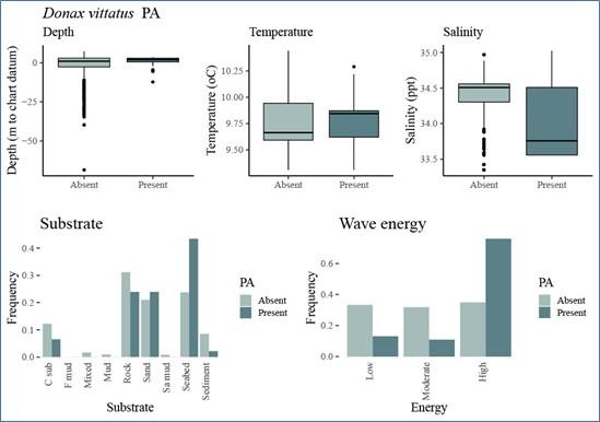
Figure 5 Donax vittatus, environmental association tests based on presence absence plots for key factors that determine habitat suitability and that were used in the model.
Click for a full description
Boxes within boxplots for depth, temperature and salinity presence/absence show the range from the lower to the upper quartile, with lines within boxes representing the median values. Whiskers stretch to 1.5 the interquartile range and points represent outliers beyond this range. Bar charts for substrate and wave energy presence/absence show the frequency of records for each category within these variables for presence and absence data separately. Scatter plots are used for depth, temperature and salinity abundance comparisons. Box plots were built for substrate and wave energy abundance data in exactly the same manner as for depth, temperature and salinity presence/absence data, with boxes, whiskers and points representing the same summary statistics.
Five plots displaying presence and absence records for Donax vittatus. The first plots are three box and whisker plots showing presence and absence in relation to depth, temperature and salinity. The final two plots are histograms mapping the frequency of presence and absence records against substratum and energy.
Species presence in unsuitable habitats
The presence of species in habitats which were considered not to be suitable may either reflect issues with survey data and coverage or point to the existence of habitat mosaics or small areas of suitable habitat within unsuitable habitat. Examples include the presence of infaunal bivalves recorded in areas assigned to rock; this may reflect misclassification of habitats or be due to the presence of sediment veneers or patches of sediment within rock. Species in some instances may also be transported into unsuitable habitats. The low numbers of records and surveys could conceivably bias results.
Biotope analysis
The key outputs of the biotope analysis are the accompanying Excel spreadsheet (showing species/biotope associations) and the mapped outputs (in STR Annexes 3 to 6). Deep sea and pelagic water column habitats were not considered. For remaining habitats, from Level 3 (broad-scale habitats) to Level 6 (sub-biotopes) of the UK Marine Habitat Classification, the spreadsheet identifies if examples of the habitat might contain specific seaduck prey. This work was used within the project to identify relevant biotopes for principal prey species. It could be applied to support evaluation of likely prey species distribution and availability for any areas with habitat maps that can be related to the UK Marine Habitat Classification.
The number of relevant biotopes varies between the prey species. Some species (D. vittatus, L. vincta and M. helicinus) were only reported as characterising single biotopes, while other prey species such as M. edulis were recorded in a wide range of biotopes. These prey species were also matched in the spreadsheet to the relevant seaduck species. Broadscale habitats (Level 3) and Level 4 biotope complexes that do not have principal prey species recorded, but which have child biotopes that do, were identified as containing prey. To identify whether intertidal mapping might be appropriate for species and biotopes we identified species that are strongly associated with intertidal habitats.
Examples of mapped outputs based on biotope analysis are shown in Figure 6 for D. vittatus; all prey species maps are provided in STR Annexes 3 and 4.
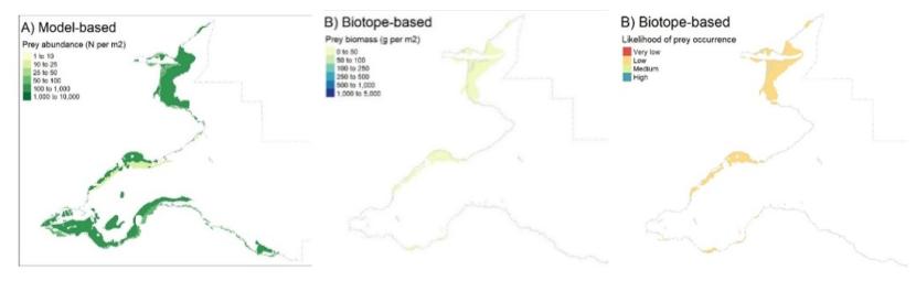
Figure 6 Donax vittatus OFFSABC SPA maps derived from biotope analysis (abundance, biomass and likelihood)
Click for a full description
Three maps of the Outer Firth of Forth and St Andrews Bay Complex SPA showing the biotope based predictive maps, respectively these map the predicted abundance, biomass and likelihood of occurrence of Donax vittatus. For each map the predicted areas are the same and the predicted level of abundance, biomass and likelihood of occurrence are not predicted to vary across the site. The species is predicted to occur in the coastal fringes of the site. The light green shading in the abundance map indicates that the predicted abundance is low where this species is predicted to occur, with between 1-10 individuals predicted in each square metre. This species is relatively small as indicated by the predicted low biomass of between 1-50g in each square metre. Likelihood of occurrence is assessed as low in the predicted suitable habitats.
Overview of outputs for prey species
Astarte elliptica
A. elliptica was recorded in 33 surveys (Table 5), with 116 presence records and 2,844 absences. There were 13 records of presence/absence within the target SPAs and no records of abundance, although there were 36 abundance records from outside the SPAs.
The environmental association tests (STR Figures 2.1 and 2.2) indicate considerable overlap over the assessed environmental variable gradients. This species was more frequently recorded in sands than other habitat types and in areas of low wave energy. The abundance records indicate this species was found in deeper areas, with high abundances recorded below 25m, and in full salinity. Substrate preferences were relatively broad with highest abundances in areas of moderate wave energy, which differs from the presence/absence records.
Modelled probability of occurrence was associated with the interaction of depth and substrate type plus wave energy (Table 11). Abundance was associated with salinity plus substrate type and wave energy. There were no data to test the species model predictions within the target SPAs. The deviance measures suggest that the model does not perform well at predicting presence and absence or abundance and therefore the results should be interpreted with caution.
This species is not a characterising species of any biotope and therefore could not be included in the mapping based on biotope analysis. Mapping of the species model outputs (STR Figures 3.1 to 3.3 and 4.1 to 4.3) predicted A. elliptica to occur in relatively small, deeper areas of the Moray Firth SPA and to occur over wider areas in the OFFSABC SPA in areas of sand and sandy mud but with very low likelihood of occurrence.
Little evidence was found in the evidence review (Annex 8 in STR) for habitat preferences and tolerances of this species and the habitat suitability predictions of the model could not be evaluated.
Cerastoderma edule
C. edule was recorded in 176 surveys with 310 presence records and 4,229 absence records. There are relatively few records of C. edule presence/absence within the target SPAs (77). There were 349 abundance records outside of the target SPAs and very few records (5) within the sites (Table 5).
The environmental association tests (STR Figures 2.3 and 2.4) found that for most variables the range where the species was absent overlapped with the ranges in which it was present, with the exception of depth; no records were found for C. edule below 100m. C. edule was mostly present in the shallow subtidal and low intertidal, as reflected in the habitat maps which predict presence in the intertidal. It was most abundant just below chart datum and while abundance information was found for some habitats deeper than 75m these were records of low abundance. However, abundance data varied considerably at the same reported depths. Median salinity values for presence data were approximately 33.9 for presence and 34.3ppt for absence data. There appeared to be no clear relationship between abundance and either salinity or temperature. C. edule tended to be found on muddy, sandy or mixed sediments with the most presence records on muddy sediments and highest abundances in sandy sediments. Numbers of presence and absence records were similar to each other across different wave energy categories, but C. edule was more likely to be present and more abundant in areas of low wave energy.
Modelled probability of species occurrence was associated with depth, temperature and substrate type, while abundance was associated with depth, temperature, substrate type and wave energy (Table 11). As suggested by the overlap in presence and absence data across environmental gradients, model performance tests suggest that the models have poor predictive ability.
The comparison of mapped outputs from the species model (STR Figures 3.4-3.6 and 4.4-4.6) and biotope analysis approaches (STR Figures 3.7-3.9 and 4.7-4.9) indicate that there are considerable differences between the two approaches. C. edule was not predicted from species models to be present in the OFFSABC SPA but was predicted to be present in the shallower fringes of the Moray Firth SPA. This tends to accord with the species’ habitat based on the evidence review that C. edule is present in the shallow subtidal. The mapping based on biotope analysis of C. edule in the two SPAs was very different, with predicted presence in OFFSABC and no overlap in areas identified as suitable habitats in the Moray Firth with those predicted by the species model. Mapping based on biotope analysis predicted that suitable habitats were present only in discrete locations but with a spatial extent greater than predicted from the species model. However, the predicted prey abundance was greater for the species models than the biotope based approach. The likelihood of occurrence was very low based on the predictive species modelling in the Moray Firth and low for the mapping based on biotope analysis in both the Moray Firth SPA and OFFSABC SPA.
The presence of C. edule within areas of substratum classified as sand and mud (with the highest number of records in mud) accords with the evidence review (STR Annex 9) as does the greater frequency of records within more sheltered areas of low wave energy. The small number of records for rock, an unsuitable habitat, points to either misclassification of sediments in surveys or seabed maps or the presence of C. edule in sediments overlying rock. The abundance records, indicate that C. edule was present in greatest numbers in the intertidal and shallow subtidal, with higher numbers in sand and muddy sand and in areas with low wave energy.
Cerastoderma glaucum
C. glaucum was identified in relatively few surveys (24). There were relatively few (43) records of presence, with this species absent from most records (1,292) and few records of abundance (10). There were 11 target SPA records of presence/absence and no abundance records.
The environmental association tests (STR Figures 2.5 and 2.6) suggest that C. glaucum is found in shallower areas (largely absent below chart datum), and is present in sheltered areas with lower wave energy and typically between 33.9 and 34.3 ppt salinity (median value for presence around 34.3 ppt). It is present in mixed, muddy and sandy habitats. For both this species and C. edule, rock habitats are not generally considered suitable and its presence in these habitats may suggest issues with the underlying survey data or seabed maps, or the presence of pockets of sediments which are suitable.
Modelled probability of occurrence was associated with interaction of depth and substrate type plus temperature (Table 11). Very limited environmental variation was shown by the small amount of abundance data available for modelling and, therefore the mean abundance value of 93.8 individuals per m2 was used. The goodness of fit measure of the presence/absence models suggested that fit was poor and the test data set was inadequate to assess model performance. The resulting outputs should therefore be treated with caution.
Comparison of mapped outputs from the species model (STR Figures 3.10-3.12 and 4.10-4.12) and biotope analysis (STR Figures 3.13-3.15 and 4.13-4.15) found that for both SPAs the predicted suitable habitats varied in location between the approaches. The species models for both sites predict higher biomass than the maps based on biotope analysis. The species model predicted high abundances of C. glaucum on the littoral fringes .of the Moray Firth SPA and the OFFSABC SPA. The biotope analysis predicted greater extents of suitable habitat, but in more restricted areas.
The species model predicted suitable habitats for C. glaucum in moderately exposed areas on sediment around the subtidal fringe of the sites. The maps based on biotope analysis suggest this species is present in small pockets of suitable habitats, some in more wave-exposed but shallow areas. C. glaucum is a subtidal species with specific habitat preferences for sheltered, stable, shallow subtidal habitats. It is not clear when assessing the evidence, whether the species modelling or biotope analysis approach more closely reflect the known habitat preferences of this species as identified by the evidence review (STR Annex 10). Likelihood of occurrence was very low across both sites for both approaches.
Donax vittatus
D. vittatus was recorded in 42 surveys, with 117 presence records and 3,595 absence records. There were 60 records of abundance from outside the target SPAs. Within the target SPAs there were 347 presence/absence records and three abundance records (Table 5).
The environmental association tests (Figure 5 and STR Figures 2.7 and 2.8) indicate substantial overlap between presence and absence records for all the assessed environmental variables, particularly salinity and temperature. However, the plots do suggest that this species is observed most frequently in shallower habitats in sand, in areas with high wave energy. Abundance records for D. vittatus indicate this species is relatively restricted to the intertidal and shallow subtidal to about 10m, in sands and areas of moderate or high energy. This species is also predicted to be present in rock habitats, which would be unsuitable. This is likely to reflect either mosaics of sedimentary habitat within rock areas, overlaying of sediments on rock or misclassification of habitat data.
The most optimal occurrence and abundance models were based on the interaction between depth and substrate type, plus wave energy (Table 11). The occurrence model for D. vittatus was one of the best performing based on the AUC measure, however the low level of deviance explained (16.9%), suggested that while the model performed well within the SPAs in general the model fit to the data was poor.
For D. vittatus, the observed distribution and the environmental variables selected for modelling accords with the habitat suitability models by Willems (2010), which found that predicted probability of occurrence is lowest in deeper waters with coarse sediments and is highest in shallow waters with fine sediments (Annex 11, STR).
Comparison of the species model (Figure 4 and STR Figures 3.16-3.18 and 4.16-4.18) and biotope analysis mapping outputs (Figure 6 and STR Figures 3.19-3.21 and 4.19-4.21) found some areas of overlap for both approaches in both SPAs. However, the maps based on the species models suggest that areas of suitable habitat are more widespread in both sites and predict higher abundance (and therefore biomass) than those based on the biotope analysis. The maps derived from biotope analysis suggest that suitable habitats exist on the littoral fringes of the Moray Firth SPA and the OFFSABC SPA. The predictive species models indicate greater extents of suitable habitats in both SPAs. Likelihood of occurrence is lower for the species model based results (generally very low through most of the extent in both sites) than for the maps based on biotope analysis.
Hydrobia spp.
The Hydrobia genus was identified in 30 surveys (Table 5). There were 64 presence records and 1,642 absence records but just two records of abundance. Within the target SPAs there were no presence/absence or abundance records.
The environmental association tests (STR Figure 2.9) showed that presence and absence overlap over environmental gradients, but that Hydrobia spp. presence records were restricted to shallow depths with no records below approximately 20m. Hydrobia spp. were more likely to be present in mud and sand and in areas of low wave energy and at lower temperatures. Median values for salinity were very similar for presence and absence data. No abundance data was available for this species.
Probability of occurrence was most likely associated with depth, temperature and substrate type. The most optimal occurrence model was based on the interaction between depth and substrate type plus temperature (Table 11). Insufficient abundance data was available for modelling and the mean abundance value (across spring and autumn samples) of 11,406 was taken from Reise et al. (1994). Tests of goodness of fit showed that model performance was poor and inadequate data were available to test the model.
The species models predicted high abundances (> 1000 individuals per m2) of Hydrobia spp. in relatively large areas of the Moray Firth SPA (STR Figures 3.22- 3.24) and OFFSABC SPA (STR Figures 4.22-4.24). As this genus is very small, the biomass maps provide useful context and the predicted biomass levels are low across both sites (0-50g/m2). For both sites confidence in the predictive mapping was very low, due to poor goodness of fit and absence of data for testing.
However, the areas predicted to be suitable did match habitat preferences identified in the evidence review (Annex 13 in STR). Hydrobia spp. were predicted to be present in shallow habitats, with sand, muddy sands and mixed sediment and in areas of moderate wave energy. In the Moray Frith in particular, this species appeared to be predicted as present where wave exposures were high, which are not considered suitable habitats (Fenchel, 1975). This factor and salinity were not included in the species models, which may have limited predictive power. Predicted occurrence also overlapped with seagrass habitats that are suitable for this genus.
No mapping based on biotope analysis was undertaken for this genus due to the absence of associated biotopes.
Lacuna vincta
L. vincta was recorded in 289 surveys, with 1,112 presence records and 14,355 absence records (Table 5). There were 179 records of abundance overall. Within the target SPAs there were 236 presence/absence records and two abundance records.
The environmental association tests (STR Figures 2.10 and 2.11) indicate that there is overlap between presence and absence records across all the assessed environmental variables. However, records suggest that L. vincta is observed more frequently in shallower habitats and lower salinities and in more sheltered habitats (low wave energy) and frequently associated with rock. It was recorded as present in all sediment types. The abundance records for L. vincta indicate this species is confined to the intertidal and shallow subtidal, with broad substratum preferences and higher abundance in areas of low wave energy (although median values were similar across the three wave exposure categories).
The most optimal occurrence model was based on the interaction between depth and substrate type. The most optimal abundance model was also based on the interaction between depth and substrate type (Table 11). Model performance, tested by the AUC, indicated the occurrence model was one of the best performing, however the goodness of fit test (deviance explained, Table 11) indicated that while the model performed well within the target SPAs the model fit to observed data was poor.
The likelihood of L. vincta occurring was very low for the Moray Firth and the OFFSABC SPAs. The species model predicted that L. vincta was present only in shallow habitats at the subtidal fringe with high wave exposure (STR Figures 3.25-3.27 and 4.25-4.27), which accords with suitable habitats identified in the evidence review (Annex 14 in STR). What is unclear is the degree to which this species is associated with sediment, as predicted by the models. L. vincta is associated with either algae, typically on rocky shores, or with seagrass which occur on a range of sediment types. While the species model performed better than others in predicting presence and absence in the SPAs, it is not clear how many, if any of these records are associated with seagrass rather than unvegetated sediments. However, checks on seagrass datapoints in the SPAs, using evidence from the National Marine Plan interactive website, showed that in both target SPAs L. vincta was predicted to be present in areas that correspond to seagrass distribution and therefore likely to be suitable habitats for this species.
L. vincta was not predicted to be present in biotopes in either the Moray Firth SPA or the OFFSABC SPA (STR Figures 3.28-3.30 and 4.28-4.30).
Limecola balthica
L balthica was recorded in 116 surveys, with 619 presence records and 5,810 absence records (Table 5). There are 294 records of abundance overall. Within the target SPAs there were 128 presence/absence records and one abundance record.
The environmental association tests (STR Figures 2.12 and 2.13) indicate that there is overlap between presence and absence records across all the assessed environmental variables, particularly for salinity. Records suggest that the species was more often present in areas with low wave energy and sandy sediments. There were fewer records from mixed and mud sediments. The abundance records show highest abundances between 0-5m depth and at salinities around 34.5 ppt and in mixed sediments. Median values for abundance were similar across the three wave categories, but with the highest abundances at moderate wave energy.
Modelled probability of occurrence was most clearly associated with depth and substrate type (Table 11) and the most optimal occurrence model was based on the interaction between depth and substrate type, plus wave energy. Abundance patterns were associated with depth, temperature, salinity and substrate type. The most optimal abundance model was based on the interaction between depth and substrate type, plus temperature. There was no evidence to test the performance of the occurrence model (as only absence records were recorded within the SPAs) but the tests of goodness of fit (deviance explained) indicate that the model fit to observed data was poor. The predictive mapping results should therefore be treated with caution.
Comparison of mapping based on species models and biotope analysis show that, while overlapping in some parts of the SPAs, there are differences in suitable habitats identified by the two approaches (STR Figures 3.31-3.36 and 4.31-4.36). The species model indicates that L. balthica is restricted to a narrow part of the subtidal fringe in both the Moray Firth and OFFSABC SPAs, but that where it occurs it may be at relatively high biomass. The mapping based on biotope analysis predicts more discrete patches of relatively small extent and with lower predicted biomass in both the Moray Firth SPA and OFFSABC SPA. For both sites and approaches the likelihood of prey occurrence is very low.
Mapping based on biotope analysis predicted L. balthica as present in areas of sediment (no detailed information on substratum type) in both SPAs. The species model however, predicted L. balthica as present predominantly in shallow sands in the Moray Firth and sands affected by riverine flows, although salinity variation in habitats is not apparent from the mapped salinity (STR Figure 1.8). The mapped distribution based on the species model was considered to represent suitable habitats for this species, which has broad tolerances for sediment substratum and salinity but which is predominantly an estuarine, intertidal or very shallow subtidal species found within muds and sands (STR Annex 15).
Macoma spp.
This genus was recorded in nine surveys (Table 5). There were 49 presence records and 3,331 absence records, but no abundance records. Within the target SPAs there were three presence/absence records.
The environmental association tests (STR Figure 2.14) indicate that there is overlap between presence and absence records across all the assessed environmental variables, although records suggest that Macoma spp. were not recorded below 50m. Macoma spp. were more often present on mud than other substratum types and in low wave energy environments. In summary, Macoma spp. appear to favour shallow, low energy, muddy habitats.
Probability of occurrence was most clearly associated with depth, salinity, wave energy and substrate type. The most optimal occurrence model for Macoma spp. was based on the interaction between depth and substrate type, plus salinity plus wave energy (Table 11). No data were available related to abundance and therefore the mean abundance value of 1 was taken from the lower bound of the corresponding SACFOR entry in Table 10, based on a SACFOR estimate obtained from the JNCC website. There was no suitable data to assess model performance within the target SPAs. However, the tests of the occurrence model goodness of fit (deviance explained) was better than for many other species, although still relatively poor.
Comparison of maps based on the species modelling and biotope analysis approaches was not possible, as Macoma spp. were not predicted to be present in biotopes in either the Moray Firth SPA or the OFFSABC SPA. In the OFFSABC SPA (STR Figures 4.37-4.39) suitable predicted habitats for Macoma spp. included coarse, mixed and sandy muds or muddy sands and in the Moray Firth SPA (STR Figures 3.37-3.39) coarse and mixed sands. In both sites predicted biomass was low (0-50 g/m2). Likelihood of prey occurrence was assessed as high for most of the predicted suitable habitats in both sites, but with some areas of very low likelihood of occurrence.
Margarites helicinus
M. helicinus was recorded in 73 surveys and there were 181 presence records and 4,221 absence records (Table 5). There were five records of abundance. Within the target SPAs there were 67 presence/absence records and no abundance records.
The environmental association tests (STR Figure 2.15) indicate that there is overlap between presence and absence records across all the assessed environmental variables, although records suggest that this species tends to occur in shallow habitats and on rock and in areas of low wave energy.
Modelled probability of occurrence was most clearly associated with depth, salinity and wave energy. The most optimal occurrence model was based on the interaction between depth and wave energy, plus salinity (Table 11). Insufficient abundance data was available for modelling and the mean abundance value of 10 was taken from the lower bound of the corresponding SACFOR entry in Table 10, based on the levels of abundance shown in the training data. Tests of model performance and goodness of fit (Table 11) indicate that model performance was poor and that the outputs should be treated with caution.
Comparison of the species model and biotope analysis mapping outputs (STR Figures 3.40-3.45 and 4.40-4.45) showed that the species model approach predicted that far greater extents of both the Moray Firth SPA and OFFSABC SPA were suitable for M. helicinus than the biotope analysis approach, which was based on the presence of infralittoral rock with high wave energy. The species model and biotope analysis outputs both indicate that the likelihood of occurrence is very low. While the species model prediction of the presence of M. helicinus in wave exposed areas was in agreement with evidence found in the evidence review (STR Annex 17), the model was considered unrealistic in terms of the substratum, based on known preferences for hard substratum and particularly kelps, rather than sediment habitats.
Mya arenaria
M. arenaria was identified in 139 surveys, with 70 presence records and 3,546 absence records (Table 5). There are 14 records of abundance overall. Within the target SPAs there were 697 presence/absence records and eight abundance records.
The environmental association tests (STR Figures 2.16 and 2.17), indicate that there is overlap between presence and absence records across all the assessed environmental variables, particularly for salinity. However, records suggest that the species was present in shallower areas, those with low wave energy and those where temperatures were higher, with greater abundances where average temperatures were above 10oC. Records also suggest that sand sediments were preferred with fewer records from mixed and mud sediments. Abundance records suggest that M. arenaria was more abundant in shallower areas, although it does also occur in deeper areas, and in areas where wave exposure is lower but has relatively broad tolerances for sediment habitats.
The most optimal occurrence model (Table 11) was based on the interaction between temperature and substrate type, plus depth and the most optimal abundance model was based on temperature. Tests of model performance and goodness of fit (Table 11) indicate that model performance was poor and, whilst the abundance predictions were highly correlated with actual abundance in the test data set, the outputs should still be treated with caution.
Comparison of mapped outputs based on the species model and biotope analysis approaches (STR Figures 3.46-3.51 and 4.46-4.51), found these to be very different for both SPAs. The extent of suitable habitat predicted by the species model far exceeds that suggested by the biotope analysis approach. The species model approach is considered to more accurately reflect suitable habitat as the evidence review (Annex 18, STR) indicates that M. arenaria is found subtidally and in the intertidal on muddy sands and mixed sediments and these habitats are widespread in both SPAs. However, the species model approach is also considered to overestimate habitat extent as this species is predominantly found in intertidal and shallow subtidal habitats, rather than the deeper habitats predicted by the abundance model.
Likelihood of occurrence was assessed as low for the approach based on biotope analysis in the OFFSABC and Moray Firth but the predicted likelihood based on the species model varies from very low to high in both sites.
Mytilus edulis
M. edulis was recorded in 436 surveys and there were 3,290 presence records and 18,442 absence records (Table 5). There are 623 records of abundance overall. Within the target SPAs there were 211 presence/absence records and no abundance records.
The environmental association tests (STR Figures 2.18 and 2.19) indicate that there is overlap between presence and absence records across all the assessed environmental variables. However, records suggest that M. edulis is present more frequently in shallower areas, areas with low wave energy and on rock, although this species was also present on sediments. The abundance records for M. edulis indicate that M. edulis has wide habitat tolerances with high abundances recorded across the assessed environmental gradients. However, it was less abundant at salinities below approximately 33.5 ppt, below 40m depth and at average temperatures below 10°C.
Probability of occurrence was only clearly associated with depth. The most optimal occurrence model was based on the interaction between depth and substrate type, however, results for substrate type were likely to have been impacted by sampling bias as they suggested low occurrence in rock substrate, which is a well-known habitat for this species (Table 11). Previous studies have found similar biased distribution patterns for M. edulis as rock is poorly sampled by infaunal grabs and therefore under-represented in sampling (Darr et al., 2014). Abundance showed a similar pattern to occurrence.
We therefore modelled M. edulis based solely on data from a video and photo survey carried out along the Dorset Coast by the Dorset Wildlife Trust, a survey method more suited to sampling an epibenthic species that frequently occurs on hard substrata, than grab sampling, which is likely to occur more often within the full data set. Analysis of this data set demonstrated that the only environmental factor associated with M. edulis abundance was substrate type, with ‘Rock’ showing a relatively high likelihood of having ‘Super abundant’ or “Abundant’ M. edulis counts (Likelihood of 0.54 compared to mean likelihood of 0.08). Apart from ‘Absent’ other abundance categories were very rare. No other substrate type had a likelihood of high M. edulis counts. Therefore, M. edulis abundance was modelled at 100 individuals per m2 in the presence of rock when it was predicted to be present.
Comparison of the species model and biotope analysis mapping outputs (STR Figures 3.52-3.57 and 4.52-4.57) showed that the species model approach and the biotope analysis produce relatively similar outputs for the Moray Firth SPA and the OFFSABC SPA, as both approaches are based on the presence of rock to indicate suitable habitats.
For the Moray Firth SPA, the species model predicted higher abundances of M. edulis than the biotope analysis and the likelihood of occurrence was medium. For the biotope analyses predicted abundance was lower and less uniform due to the underlying biotopes and likelihood of occurrence varied from medium to low.
The mapping outputs from the OFFSABC SPA are similar to those from the Moray Firth SPA, with higher abundances predicted from the species model and medium likelihood of occurrence predicted across the site and the biotope analysis predicting lower abundance and variable likelihood of occurrence (medium or low). A key difference between the approaches for the OFFSABC SPA, is that the species model predicted a greater extent of suitable habitat in the central and southern parts of the Firth of Forth corresponding to areas of rock. Examination of the mapped environmental variables suggests that this is due to areas of rock exposed to low wave energy being included as suitable habitat by the species models approach but not the biotope analysis. Filter feeders such as M. edulis require water movement to supply food particles. In areas of low wave energy and low current speeds populations may not receive sufficient food. It is not possible to identify which model is most accurate without ground truthing to determine suitable habitats, although it is possible that for the OFFSABC SPA the species model overestimates the extent of suitable habitat.
Comparison with the literature review suggests that the species model outputs may underestimate occurrence as M. edulis is known to be present on a wide range of substratum (Annex 19 in STR) and may be more widespread in both sites. However, the biotope review found that M. edulis was only abundant or common on rock biotopes or mussel beds, not sedimentary habitats.
Spisula subtruncata
S. subtruncata was recorded in 74 surveys with 713 presence records and 5,741 absence records (Table 5). There were 257 records of abundance overall. Within the target SPAs there were 230 presence/absence records and two abundance records.
The environmental association plots (STR Figures 2.20 and 2.21) indicate that there is overlap between presence and absence records across all the assessed environmental variables, although records suggest that it tended to be present in shallow habitats. There were a few records of this species in rock habitats, which are generally considered unsuitable, but it is typically found within sediments including mixed and muddy sediments with higher frequencies on sand and with broad tolerances for wave energy. The abundance records suggest higher abundances in shallower areas (from chart datum to 25m), although this species has broad depth tolerances. Higher abundances were generally found in areas with moderate wave energy.
Modelled probability of occurrence was most clearly associated with depth, substrate type and wave energy. The most optimal occurrence model was based on depth and substrate type (Table 11). Abundance was associated with depth, temperature, substrate type and wave energy. The most optimal abundance model was based on temperature, substrate type and wave energy. The AUC test for the occurrence model shows that model performance was poor. Test data was inadequate to test the performance of the abundance model. Modelled outputs should therefore be treated cautiously.
The comparison of mapped outputs from the species model and biotope analysis approaches (STR Figures 3.58-3.63 and 4.58-4.63) showed that the distributions were predicted to be quite different. This species was only associated with one biotope, infralittoral muddy sands, hence the maps derived from the biotope analysis for both the Moray Firth and the OFFSABC SPAs suggested that suitable habitats for S. subtruncata were restricted to the subtidal fringe, whereas the species model outputs for both sites suggested that areas of suitable habitat correspond to deeper areas of sandy mud/muddy sand. Comparison with the literature review outputs (STR Annex 20) indicated that while the species model aligned with evidence that S. subtruncata was positively correlated with mud content, it was possible the species model underestimated suitable areas of habitat in the Moray Firth and OFFSABC SPAs, as this species can also occupy subtidal sand habitats which occur extensively across both sites.
Seaduck prey maps
Following the production of the prey species maps, maps for total principal prey taxa abundance and biomass, derived from the species modelling and biotope analysis approaches, were produced for each seaduck species. Full results for all seaduck species within the Moray Firth SPA and OFFSABC SPA are available in Annexes 5 and 6 respectively of the STR. Examples of combined principal prey maps derived from both approaches for the Moray Firth SPA are shown for common scoter (Figure 7) and long-tailed duck (Figure 8).
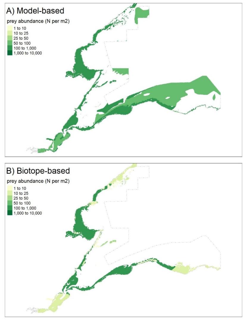
Figure 7. Common scoter, mapped outputs for the Moray Firth SPA showing A) predicted abundance based on species models and B) predicted abundance based on biotope analysis.
Click for a full description
The figure consists of two maps of the Moray Firth SPA showing the predicted combined abundance of principal prey for common scoter. Figure A provides the predictive model-based mapping and Figure B the biotope-based mapping. The abundance in both maps is described using colour shading based on a colour scale ranging from light to dark green scaled over six categories. The lowest abundance of 1-10 principal prey species is shown as the lightest green and the highest abundances of 1,000-10,000 presented as the darkest.
Both maps predict that prey abundance varies across the site but both methods also identify similar areas of suitable habitat around the landward boundaries. The predictive model map indicates larger areas of suitable habitat for prey in the south western part of the site in the area between Nairn and Portsoy.
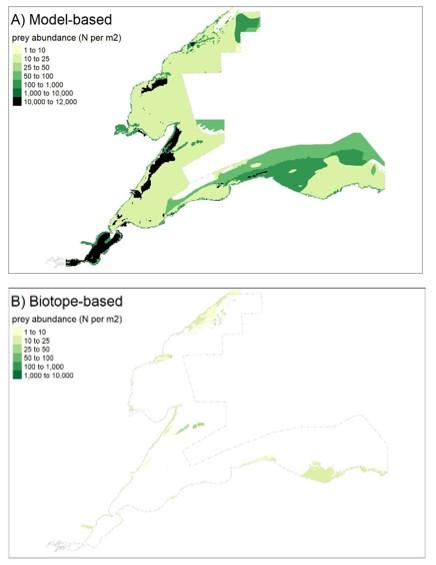
Figure 8. Long-tailed duck, mapped outputs for the Moray Firth SPA showing A) Species model-based combined principal prey abundance predictions and B) Biotope-based predictions of combined principal prey abundance.
Click for a full description
The figure consists of two maps of the Moray Firth SPA showing the predicted combined abundance of principal prey for long-tailed duck. Figure A provides the predictive species model-based mapping and Figure B the biotope-based mapping. The abundance in both maps is described using colour shading based on a colour scale ranging from light to dark green and black scaled over seven categories. The lowest abundance of 1-10 principal prey species is shown as the lightest green and the highest abundances of 10,000-12,000 presented as the darkest. The species model-based approach predicted extensive suitable habitats across the site with varying prey abundance.
These mapped outputs exemplify the differences across seaduck species between the outputs based on species models and those based on biotope analysis. It should be noted that all maps discriminate between areas of greater and lower abundance of principal prey (and therefore, biomass which is based on abundance conversion) and between likelihood of occurrence. These areas also differ between seaduck species, suggesting that both approaches provide an opportunity to identify potential foraging areas, as prey availability is not uniform across the site.
For three contrasting seaduck species, the combined principal prey species model and biotope analysis mapping outputs were compared against observed seaduck species’ distributions within the two SPAs, as described in the relevant Site Selection Documents (NatureScot, 2016 and NatureScot and JNCC, 2016). This provides a sense check of the prey mapping outputs and demonstrates how the evidence review outputs and the mapping outputs can be evaluated to identify potentially suitable habitats for seaduck principal prey. As there are no ground truthing data to confirm the predictions, the results can only be considered as indications of where suitable habitats may be present.
Common eider
Mapped prey species: A. elliptica, C. edule, L. balthica, M. edulis, S. subtruncata
Moray Firth
Common eider are distributed throughout most of the site between Brora and Portsoy. The relative density maps of common eider suggest areas of highest density observed around Lossiemouth and at the entrances of the inner Moray Firth and the Dornoch Firth around Portmahomack Bay (Figure 9).
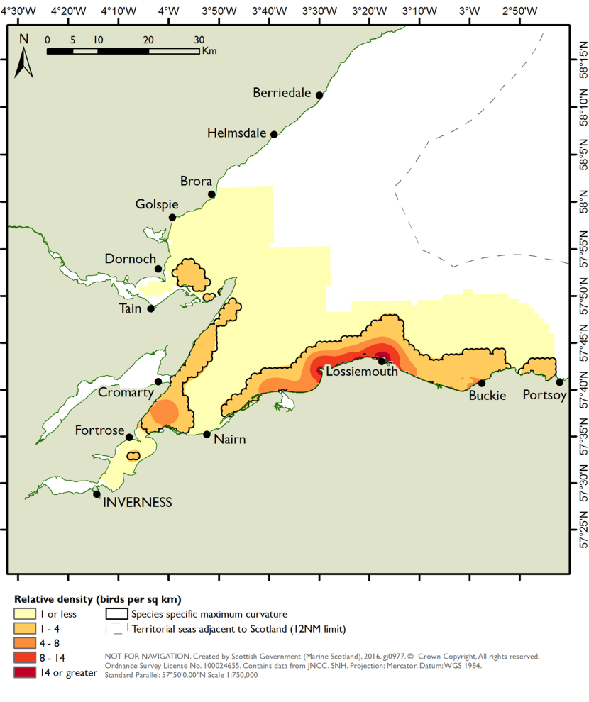
Figure 9. The distribution of common eiders in the Moray Firth SPA.
Click for a full description
Distribution derived from aerial surveys during the winter seasons of 2001/02 to 2006/07 (NatureScot 2016). The derivation of the maximum curvature boundary is described in JNCC (2016).
The figure presents information on the distribution of common eiders in the Moray Firth SPA. The map scales the abundance of seaduck from 1 or less per square kilometre) to the greatest density of 14 or more. The information is shown as five categories as a colour coded scale to provide a heat map effect with lower densities of seaduck shown as lighter yellows and the higher densities as darker reds. Common eider are distributed throughout most of the site between Dornoch and Portsoy. The relative density maps of common eider suggest areas of high density around Lossiemouth and at the entrances of the inner Moray Firth and the Dornoch Firth.
The principal prey species modelled abundance and hence biomass mapping identified suitable prey habitats in patches throughout the SPA. The maps (STR Figures 5.1-5.3) indicate areas with high biomass around the Lossiemouth area corresponding to the highest density of common eider. Areas predicted to have high biomass of prey also occurred at the mouth of the inner Moray Firth within the SPA and intertidally within Loch Fleet, which is outwith the SPA boundary.
Assessment of individual prey species model maps indicates that the inshore high prey biomass around Lossiemouth (at the coastal fringe where the highest abundances of common eider were observed) was contributed by M. edulis (STR Figure 3.53), C. edule (STR Figure 3.5) and L. balthica (STR Figure 3.32).
At Portmahomack Bay (Dornoch Firth) the high biomass of prey was supported principally by L. balthica with smaller extents of suitable habitat supporting C. edule; and S. subtruncata.
Areas identified as suitable habitat for prey species within the Inner Moray Firth, where lower abundances of common eider were observed, were based on M. edulis and L. balthica on the northern coastal fringe and the C. edule and L. balthica species model predictions for the southern coastal fringe.
Within the SPA away from the coastal boundaries, areas predicted to be suitable for prey were based on the species models for A. elliptica and S. subtruncata.
The mapping based on biotope analysis (STR Figures 5.4-5.6) predicted high levels of biomass throughout the coastal fringe and therefore did not discriminate between habitats, suggesting that much of the site supports high prey biomass. The high prey biomass is not predicted to be supported by C. edule or A. elliptica (no map derived from biotope analysis), but is contributed to partially by pockets of biotopes characterised by M. edulis (STR Figure 3.56) and L. balthica (STR Figure 3.35) with the main driver of biomass estimates being S. subtruncata (STR Figure 3.62) characterised biotopes.
OFFSABC
High densities of common eiders (up to 200 or more per square kilometre (sq km) occur around the entrance to the Firth of Tay with lower densities (of 10-50 birds per sq km) present throughout a large proportion of the central and northern Firth of Forth (Figure 10).
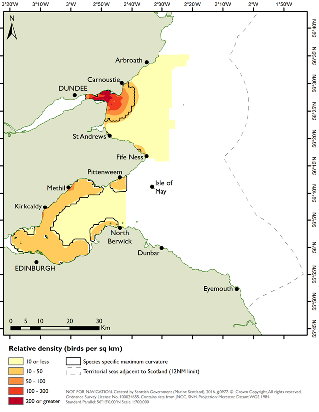
Figure 10. The distribution of common eiders in the Outer Firth of Forth and St Andrews Bay Complex SPA
Click for a full description
Distribution derived from aerial surveys during the winter seasons of 2001/02-2004/05 (NatureScot & JNCC, 2016). The derivation of the maximum curvature boundary is described in JNCC (2016).
The figure presents information on the distribution of common eiders in the Outer Firth of Forth and St Andrews Bay Complex SPA. The map scales the abundance of seaduck from 10 or less per square kilometre, to the greatest density of 200 or more. The information is shown as five categories as a colour coded scale to provide a heat map effect with lower densities of seaduck shown as lighter yellows and the higher densities as darker reds. High densities of eiders (up to 200 or more per square kilometre) occur around the entrance to the Firth of Tay with lower densities (10-50 birds per square kilometre) present throughout a large proportion of the central and northern Firth of Forth.
The mapping of prey biomass based on species modelling (STR Figure 6.2) identified areas of suitable habitat, but with relatively low prey biomass, consistent with the areas of high eider density within the Firth of Tay. However, it did predict high abundance and biomass of principal prey species throughout the Firth of Forth. The mapping based on biotope analysis (STR Figures 6.4-6.6) predicted suitable habitats supporting high biomass of principal prey in St Andrews Bay and the Firth of Tay, in addition to northern parts of the Firth of Forth, with lower prey biomass in the southern part and only small extents of suitable habitat within the central area.
The mapping of suitable habitats within the key common eider areas derived from species modelling was based on two principal prey. Biomass estimates within the Firth of Tay were based on the L. balthica predictive model (STR Figure 4.32) while in the Firth of Forth, away from the immediate coastal fringe, S. subtruncata was the species predicted to contribute to the mapped biomass (STR Figure 4.59).
The mapping based on biotope analysis indicate that C. edule contributed to the prey species biomass in the southern part of the Firth of Forth (STR Figure 4.8) but not the areas of high prey density in the northern part or St Andrew’s Bay. M. edulis (STR Figure 4.56) and L. balthica biotopes (STR Figure 4.35) were not present in the main areas used by common eider and the main driver of predicted biomass was S. subtruncata (STR Figure 4.62). There was no biotope map for A. elliptica, so this was not a driver of prey distribution as indicated by biotope analysis.
Long-tailed duck
Mapped prey species: Hydrobia spp, L. vincta, L. balthica, Macoma spp, M. helicinus, M. arenaria, M. edulis;
Moray Firth
Long-tailed duck are abundant in the Moray Firth and widely dispersed (Figure 11). High densities were recorded in Spey Bay and along the south coast of the outer Moray Firth west to Nairn, within the inner Moray Firth, and at the mouth of the Dornoch Firth.
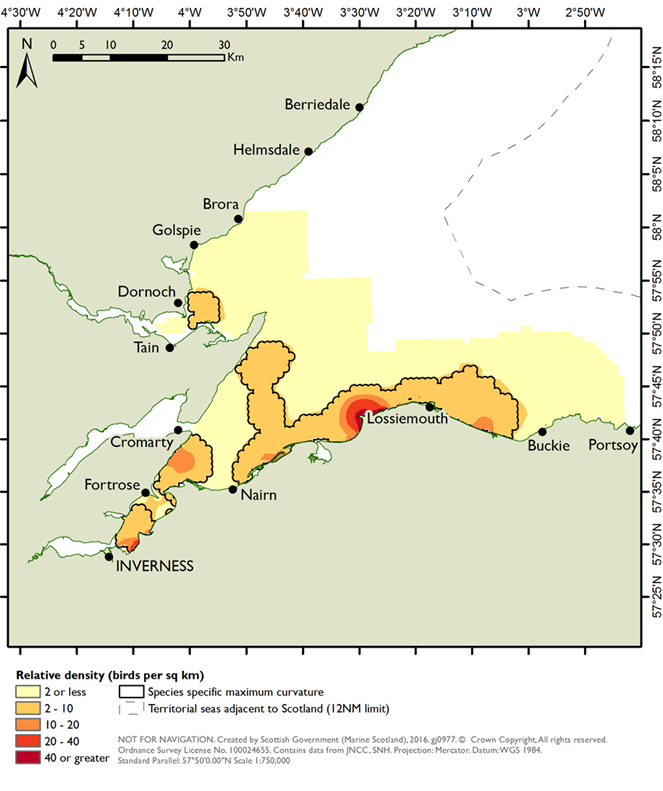
Figure 11. The distribution of long-tailed duck in the Moray Firth SPA
Click for a full description
Distribution derived from aerial surveys during the winter seasons of 2001/02 to 2006/07 (NatureScot 2016). The derivation of the maximum curvature boundary is described in JNCC (2016).
The figure presents information on the distribution of long-tailed duck in the Moray Firth SPA. The map scales the abundance of seaduck from 2 or less per square kilometre to the greatest density of 40 or more. The information is shown as five categories as a colour coded scale to provide a heat map effect with lower densities of seaduck shown as lighter yellows and the higher densities as darker reds. Long-tailed duck are abundant in the Moray Firth and widely dispersed. High densities were recorded in Spey Bay and along the south coast of the outer Moray Firth to Nairn, within the inner Moray Firth and at the mouth of the Dornoch Firth.
The species modelling approach predicted high prey biomass in areas that correspond to higher densities of seaduck in Spey Bay and inner Moray Firth and parts of the entrance to the Dornoch Firth, and appears to predict suitable habitats for prey that were not identified by the biotope analysis approach (Figures 8A and 8B). In contrast, the suitable habitats for prey predicted by the biotope analysis approach did not correspond to areas where long-tailed duck densities were greater.
The principal prey species that contribute to the predicted biomass in each area were assessed for both approaches. Within the Inner Moray Firth and the smaller areas, predictive species modelling identified areas of high prey abundance and biomass of M. arenaria, Hydrobia spp. and L. vincta (STR Figures 3.46, 3.22 and 3.25 respectively). The contribution of Hydrobia spp. to biomass was low given the small size of this species (STR Figure 3.23). L. balthica (STR Figure 3.31) was also predicted to be present in a small area corresponding to higher long-tailed duck density. Predicted areas of high abundance of M. arenaria also underpinned areas of high predicted abundance of prey by the model approach in southern, northern and central areas, however, these did not overlap with high abundance of long-tailed duck and the concerns outlined above should be noted: that the species model approach potentially over estimated areas of suitable habitat for M. arenaria in the Moray Firth.
From Nairn to Spey Bay the species models predicted L. vincta and L. balthica to be present in the coastal fringe, with more extensive areas of suitable habitat for M. arenaria (STR Figures 3.25, 3.31 and 3.46). At the entrance of the Dornoch Firth, suitable habitats for L. vincta and L. balthica are present and these species are predicted to occur at high abundances.
M. helicinus was predicted to be present throughout the Moray Firth SPA (STR Figure 3.40) but this model was not considered to be realistic and did not discriminate between unsuitable and suitable habitats.
No maps based on biotope analysis could be produced for Macoma spp, (no associated biotopes), or L. vincta and Hydrobia spp (associated biotopes not present). Neither these nor the seagrass bed habitats that occur in the SPA appear to underpin the observed high density areas for long-tailed duck in the Moray Firth SPA. The biotope analysis approach (Figure 8B) predicted that M. arenaria, M. helicinus and L. balthica (STR Figures 3.49, 3.43 and 3.34 respectively), were absent from areas where long-tailed duck were observed at high densities. M. edulis was predicted to be present around Lossiemouth (STR Figure 3.55) but at comparatively low abundances.
OFFSABC
Notable densities of long-tailed duck are found across the central and northern Firth of Forth and the Firth of Tay between St Andrews Bay and Carnoustie (Figure 12).
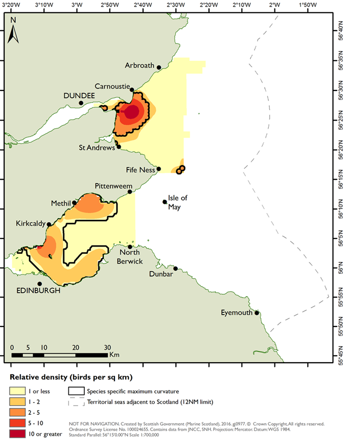
Figure 12. Distribution of long-tailed duck in the Outer Firth of Forth and St Andrews Bay Complex SPA
Click for a full description
Distribution derived from aerial surveys during the winter seasons of 2001/02-2004/05 (NatureScot & JNCC, 2016). The derivation of the maximum curvature boundary is described in JNCC (2016).
The figure presents information on the distribution of long-tailed duck in the Outer Firth of Forth and St Andrews Bay Complex SPA. The map scales the abundance of seaduck from 1 or less per square kilometre, to the greatest density of 10 or more. The information is shown as five categories on a colour coded scale to provide a heat map effect with lower densities of seaduck shown as lighter yellows and the higher densities as darker reds. Notable densities of long-tailed duck are found across the central and northern Firth of Forth and the Firth of Tay between St Andrews Bay and Carnoustie.
The species modelling approach indicates moderately high prey biomass available in the Firth of Tay and high prey biomass in the southern part of the Firth of Forth (STR Figure 6.20). Highest prey abundances predicted by the species models, therefore do not correspond directly with the highest densities observed for this seaduck, particularly in the area around Methil, but the models do predict that suitable habitats for prey species are found in areas where high long-tailed duck densities are observed.
The species prey maps were checked to identify prey species that account for the biomass patterns observed in areas corresponding to high densities of long-tailed duck. The modelled prey species distributions show that the biomass in the Firth of Tay is not contributed by M. edulis or Macoma spp (STR Figures 4.53 and 4.38), but by L. vincta (STR Figure 4.26), where it may be associated with seagrass beds, together with L. balthica (STR Figure 4.32) at moderate biomass (50-100 g/m2) and M. arenaria (100-250 g/m2). M. arenaria is the main species contributing to total modelled biomass (STR Figure 4.47). M. helicinus was predicted to be present (STR Figure 4.40) but this model was considered to have limitations (see Results).
In the central and northern parts of the Firth of Forth, M. edulis was predicted to be absent (STR Figure 4.52) but the following prey species were present: Macoma spp (STR Figure 4.38) present throughout the area at low biomass; low biomass of M. helicinus (STR Figure 4.41, but note low confidence in this model); and low and patchy contribution of M. arenaria (STR Figure 4.47). The biomass in the southern Firth of Forth is based on the predictive models for L. vincta (STR Figure 4.26) and Macoma spp (low biomass, STR Figure 4.38), with low and patchy contribution of M. arenaria (STR Figure 4.47). S. subtruncata was predicted to be present throughout the Firth of Forth at high biomass (STR Figure 4.59).
No maps based on biotope analysis could be developed for Hydrobia spp. or Macoma spp. and biotopes associated with L. vincta were not present in the OFFSABC.
The biotope-based maps (STR Figures 6.22-6.24) identified small areas of suitable habitat for prey species within the areas where long-tailed duck occur at higher densities. The biomass in the Firth of Tay corresponds with patches of biotopes that support M. arenaria (STR Figure 4.50). The biomass in the Firth of Forth resulted from predicted biomass of L. balthica (southern and central areas) (STR Figure 4.35) and M. arenaria (small patches near Methil and the centre of the Firth of Forth) (STR Figure 4.50) within suitable biotopes. The biotope analysis also predicted extensive areas of suitable habitat for prey that did not correspond to the observed areas of higher density of long-tailed duck.
The areas identified as supporting high biomass of prey differed between the two approaches: more extensive areas of suitable prey habitat were predicted by the combined species model mapping. As the prey species: Hydrobia spp., Macoma spp and L. vincta are not associated with any biotopes in the UK Marine Habitat Classification the biotope analysis is based on fewer species, which may partly account for the smaller area of suitable prey species habitat predicted based on this approach.
Common scoter
Common scoter: Mapped prey species: C. edule, C. glaucum, D. vittatus, Ensis leei (not modelled and no associated biotopes); L. balthica, Macoma spp, M. arenaria, M. edulis, S. subtruncata
Moray Firth
Scoter species form dense flocks and so were less widely distributed than other seaduck in the Moray Firth. They were generally concentrated close inshore between Burghead and Nairn, in Spey Bay and around the mouth of Loch Fleet (Figure 13). Flocks of scoter are also regularly recorded slightly further offshore at the mouth of the Dornoch Firth (Graham and Thompson, 2023; Patterson, 2021).
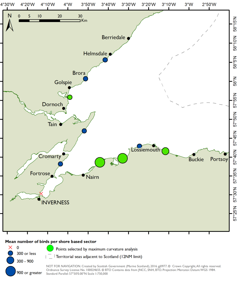
Figure 13. The distribution of common scoter in the Moray Firth SPA.
Click for a full description
Distribution derived from shore-based counts during the winter seasons 2001/02 and 2005/06 (NatureScot, 2016). Point symbols represent the relative number of common scoter in each count sector. Count sectors that warranted inclusion within the proposed site boundary were identified by maximum curvature (see JNCC (2016).
The figure presents information on the distribution of common scoters in the Moray Firth SPA. The map shows the distribution as blue or green circles indicating the mean number of birds with the size of the circle indicating the number of birds on a three point scale ranging from 300 or less to 900 or more. Green circles show sectors with the highest relative count that warranted inclusion within the proposed SPA boundary and were identified by maximum curvature. Scoter species form dense flocks and so were less widely distributed than other seaduck in the Moray Firth. They were generally concentrated close inshore between Burghead and Nairn, in Spey Bay and around the mouth of Loch Fleet.
Both the species modelling and biotope analysis approaches (Figure 7 and STR Figures 5.7-5.12) predicted high prey species biomass corresponding to areas where high common scoter counts were observed. Prey species supporting the biomass estimates were similar for both approaches but with some minor differences in extent or biomass.
The maps derived from species models predict that between Nairn and Spey Bay, C. edule (STR Figure 3.5) L. balthica (STR Figure 3.32) and M. edulis (STR Figure 3.53) underpin the predictions of high biomass on the site fringe with C. glaucum (STR Figure 3.11) predicted to be present in smaller areas in Spey Bay. S. subtruncata (STR Figure 3.59) occurs in deeper habitats. M. arenaria (STR Figure 3.47) and D. vittatus (STR Figure 3.17) were predicted to occur at high biomass with more extensive suitable habitats than the cockle species. Habitats at the entrance of and within the Dornoch Firth are predicted to support high biomass of L. balthica, C. edule and D. vittatus.
Mapping based on biotope analysis did not predict the presence of L. balthica, M. arenaria, C. edule or C. glaucum in the key areas between Nairn and Spey Bay (STR Figures 3.34, 3.49, 3.8 and 3.14 respectively). Habitats suitable for D. vittatus were predicted as present but with lower biomass than the predictions derived from species modelling (STR Figures 3.20 and 3.17). The prey biomass was supported by the high predicted biomass of S. subtruncata (STR Figure 3.62).
Biotopes suitable for D. vittatus and S. subtruncata were also predicted to occur at the mouth of the Dornoch Firth and in the intertidal habitats within and at the entrance to Loch Fleet. These species are key drivers of the biomass predicted by biotope analysis throughout the site.
OFFSABC
Densities of common scoter are generally high within the southern and northern parts of the Firth of Forth. St Andrews Bay and the mouth of the Firth of Tay are also important areas with the highest site densities (Figure 14). The mapping derived from both species modelling and from biotope analysis (STR Figures 6.7-6.12) suggested that prey biomass was high in areas corresponding with high scoter density, particularly the northern parts of the Firth of Forth and St Andrews Bay.
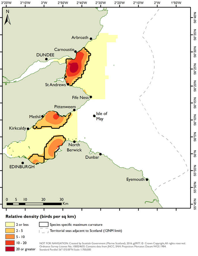
Figure 14 Distribution of common scoter in the Outer Firth of Forth and St Andrews Bay Complex SPA
Click for a full description
Distribution derived from aerial surveys during the winter seasons of 2001/02-2004/05 (NatureScot & JNCC, 2016). The derivation of the maximum curvature boundary is described in JNCC (2016).
The figure presents information on the distribution of common scoter in the Outer Firth of Forth and St Andrews Bay Complex SPA. The map scales the abundance of seaduck from 2 or less per square kilometre, to the greatest density of 20 or more. The information is shown as five categories on a colour coded scale to provide a heat map effect with lower densities of seaduck shown as lighter yellows and the higher densities as darker reds. St Andrews Bay and the mouth of the Firth of Tay are the areas with the highest site densities. Densities of common scoter are generally high within the southern and northern parts of the Firth of Forth.
The mapped outputs derived from species modelling (STR Figure 6.8) predict high prey species biomass in the areas that correspond with the highest densities of common scoter. Checks against individual prey species modelled biomass predictions found that D. vittatus (STR Figure 4.17) is the main prey species underpinning predicted biomass with habitat also predicted as suitable for some other prey species.
In St Andrews Bay and the entrance to the Firth of Tay the species underpinning the high biomass estimates are D. vittatus with moderate biomass of M. arenaria (STR Figure 4.47) and low biomass of L. balthica (STR Figure 4.32).
In the northern and southern parts of the Firth of Forth the main species supporting the high biomass estimates are D. vittatus and S. subtruncata (STR Figures 4.17 and 4.59) with extensive areas of suitable habitat for M. arenaria and more limited areas predicted to be suitable for M. edulis.(STR Figures 4.47 and 4.53). Large areas of suitable habitat for Macoma spp. were predicted, but with the species occurring at low abundance and low biomass (STR Figures 4.37 and 4.38).
The mapping derived from biotope analysis predicts high prey biomass in both the northern part of the Firth of Forth and St Andrews Bay but predicts lower prey biomass in the southern part of the Firth of Forth (STR Figure 6.11). The predictions based on biotope analysis suggest that areas of suitable habitat for principal prey are less extensive than predicted by species modelling.
In St Andrews Bay, the prey species driving the predictions based on biotope analysis are the same as for the species modelling approach. The main prey species predicted are S. subtruncata (STR Figure 4.62) and D. vittatus, but with lower biomass than the species model (STR Figure 4.20). Small areas of suitable habitat for L. balthica, occurring at low biomass (STR Figure 4.35) and M. arenaria at low abundance (STR Figure 4.49) are also predicted.
In the northern Firth of Forth the main prey species was D. vittatus (but at lower predicted biomass than the species model), with small areas of M. arenaria, and high biomass of S. subtruncata (STR Figures 4.20, 4.49 and 4.62). C. edule is predicted to occur in the southern parts of the Firth of Forth (STR Figure 4.8).
In the southern Firth of Forth the key prey species differed from the species modelling approach with biomass estimates supported by small areas of suitable habitat for L. balthica and M. arenaria at low abundance and high biomass of S. subtruncata in small areas (STR Figures 4.35, 4.49 and 4.62).
In summary for both SPAs, both the species modelling and biotope analysis approaches predicted high areas of principal prey species biomass in areas that correspond with higher densities of common scoter. The species modelling approach predicts greater extent of habitats suitable for relevant prey species throughout the SPA, (but with highest biomass in areas supporting scoter flocks), whereas the biotope analysis predictions are more restricted to the coastal fringe. Key prey species were similar for both approaches with D. vittatus, one of the main drivers for both sites, although the approaches differed in biomass predictions and extents for S. subtruncata.
Discussion
Value of approaches
The approaches to predictive mapping based on species modelling and biotope analysis were complementary but outputs require careful interpretation and consideration alongside information from the evidence review. Also, maps based on biotope analysis could not be produced for species that are not identified as characterising biotopes (Macoma spp.) or for which associated biotopes were not present in one or both SPAs (Hydrobia spp. or L. vincta).
For each principal prey species the maps derived from the species modelling and biotope analysis approaches were compared and considered in the context of information on suitable habitats gathered in the evidence review and the underlying habitat variables in both sites. This approach demonstrates that there was value in both approaches, but it was not clear which approach performed better as the outputs are not ground truthed. Given these limitations, it was considered that there were strengths and weaknesses in the results for each species but that overall both approaches were useful. The Excel spreadsheet developed for this project can in future be updated with additional prey species, as the UK Marine Habitat Classification structure has been retained and can support evaluation of likely prey species distribution and availability for other areas with habitat maps that can be related to the classification.
The mapping derived from species modelling and biotope analysis produced similar outputs for M. edulis but for many other species the results were relatively dissimilar. For some, such as S. subtruncata, M. arenaria and L. balthica these approaches identified different areas as suitable habitats, with the species model outputs considered to more realistically represent the habitats in which the species was typically found (based on the evidence review). Conversely, this was not the case for M. helicinus, where the lack of substratum category within the most optimal model meant that what are probably unsuitable habitats were included in the mapped outputs.
For some prey species, such as M. arenaria, limitations were identified with both the biotope analysis and species modelling approaches as these were considered, based on the evidence review, to underestimate and overestimate the extent, respectively, of suitable habitats.
For species with restricted biotope distributions such as L. vincta, (a characterising species for a single biotope), the use of survey data and predictive modelling provided more information than the biotope analysis approach. In the UK Marine Habitat classification, L. vincta is recorded only from infralittoral rock and this biotope was not present in the Moray Firth or the OFFSABC SPAs. However the survey data (STR Annex 2), showed that this species was recorded across a range of substrate types, including mixed, mud and sand sediments where it may be associated with seagrass The distribution of this species in both the Moray Firth SPA and OFFSABC SPA corresponded with seagrass data points, providing additional information that would not be captured solely by an approach based on biotope analysis. While caveats have already been raised around substrate, the species models appear to provide a potentially realistic habitat envelope. Similarly, Hydrobia spp. were not suitable for mapping based on biotope analysis (no characterising biotopes) but the predictive species model did indicate occurrence in areas where seagrass is present.
Comparison of outputs with observed seaduck distributions
The comparison of the combined prey species maps produced by the predictive species models and the biotope analysis (STR Annexes 3 and 4) with maps of seaduck abundance, showed that the results were variable between seaduck species and sites. Neither approach was consistently better aligned to seaduck abundance.
For common eider, both the biotope analysis and species models for the Moray Firth predicted similar areas to have high abundance of principal prey. However, although distribution was similar, the predicted extent of habitats that support higher abundances of prey species was greater for the biotope-based approach (driven by biotopes characterised by S. subtruncata) than the species modelling approach. Conversely, within the OFFSABC SPA, the outputs derived from predictive species modelling and biotope analysis were relatively different (with some overlaps). The predictive species models suggested that habitats supporting prey species were more extensive throughout the SPA. Both approaches identified suitable habitats for principal prey throughout the sites and in areas corresponding to higher abundances of seaduck.
Predicted prey maps and seaduck maps also identified comparable areas of suitable habitat with high prey and common scoter abundance within the Moray Firth and the OFFSABC SPAs. For both sites, the approaches based on species modelling and on biotope analysis predicted high prey species biomass corresponding to areas where high common scoter counts were observed. The species model approach predicted greater extent of suitable habitats throughout the SPA, whereas the maps derived from the biotope analysis were restricted to the landward boundaries.
For long-tailed duck in the Moray Firth, there was concurrence between predicted prey species models and areas with higher density of birds. In contrast, the suitable habitats for prey predicted by the biotope analysis approach did not correspond to areas where long-tailed duck densities were greater. The species model approach predicted high prey biomass in areas that correspond to higher densities of seaduck in Spey Bay and inner Moray Firth and parts of the entrance to the Dornoch Firth, and appears to predict suitable habitats for prey that were not identified by the approach based on biotope analysis.
While the mapped outputs do generally predict high principal prey biomass in areas with greater numbers of seaduck, these assessments do not identify causal relationships underlying seaduck distribution. Other factors may also influence distributions. However, the mapping approaches do appear to discriminate between suitable and unsuitable habitats for principal prey species and these appear to be valid approaches that are supported by the seaduck data. Neither approach could be judged to be superior as both approaches appear to have value.
Sources of uncertainty and limitations
There are a number of uncertainties and limitations that impact confidence in the results. These are summarised briefly in Table 12 with key points relating to specific aspects discussed below in further detail.
| Source of uncertainty/ limitations | Brief description of uncertainty or limitation | Assessed as part of project? |
|---|---|---|
| Seaduck diet evidence limitations | Limited number of studies, many international (Woodward and Humphreys, unpublished). Also, there is evidence for considerable prey switching and flexibility in prey selection for seaduck. Target prey species availability and importance may vary according to abundance and seasonal variations in sediment burying depth among other factors. | No, lack of evidence to quantify or apply. |
| Seaduck site preferences and choices | Seaduck may select areas based on factors such as lack of disturbance rather than optimal prey availability and these may limit confidence in the sense checking exercise. | No, lack of evidence to quantify or apply. |
| Principal prey evidence and data limitations | For principal prey species, the evidence base on important factors driving habitat suitability and population dynamics were not researched for some species and there was a lack of evidence and data for causal factors such as biological interactions (predation, competition). Model performances are compromised by poor quality absence data. Prey data used in the project was collected by separate surveys and at different times. Details of methods used within each survey are not available, resulting in error and bias. Species may be absent from suitable habitats and may at times be present in unsuitable habitats (due to displacement etc.) or habitat occupation may vary seasonally or over longer time scales, as reflected in the sometimes low % of occurrence for biotopes. Key factors may be site specific and vary spatially and temporally or be difficult to measure (e.g. food availability). | The impact of these on the models are not quantifiable |
| Environmental data | Limitations in data availability and data resolution. Also, many environmental variables are correlated and important factors underlying distribution such as high predation are not captured. Environmental data collected separately and at different times. | Not quantifiable. |
| Principal prey species associated with biotopes | The UK Marine Habitat Classification does not include every species recorded and species associations with individual biotopes varies, the presence of a biotope does not mean that every constituent species is present. | Not quantifiable |
| Predictions of biomass and abundance | Biomass and abundance of species is likely to vary considerably. Biomass changes over age. Abundance may also vary considerably between child biotopes within broadscale habitats and Level 4 biotopes, as shown in the supplementary Excel spreadsheet. Within biotopes of the same type the presence (occurrence) of the prey species will vary. | Uncertainty regarding biotope associations addressed by using % occurrence in biotope mapping |
Seaduck diet evidence limitations
For seaduck there is some uncertainty around diets due to the relatively limited number of studies. Many studies reviewed in the previous projects were not from the UK, and there was evidence for considerable prey switching and flexibility in prey selection. Within wintering areas, temporal dietary flexibility may be linked to prey depletion (Fox, 2003) or to seasonal preferences, for example ahead of spring migration, as has been proposed with respect to observed seasonal changes in foraging distributions and behaviours of common scoter and long-tailed duck in the Moray Firth (Patterson et al, 2022). Target species importance may vary according to a range of factors, including, among others, their abundance and seasonal variations in sediment burying depth. Seaduck may select areas based on factors such as lack of disturbance rather than optimal prey availability and these may limit confidence in the sense checking exercise.
Similarly, while efforts were made to focus on information from the UK when reviewing evidence for the principal prey taxa (Task 1), evidence for some species was relatively sparse and was supplemented by evidence from other countries. The applicability of some of this evidence is uncertain, particularly where it relates to life-history parameters that may be affected by climate, such as temperature effects on growth (relevant to review of wet weight values). In general, certain species-environment relationships are expected to be consistent, for example, sediment limitations due to burrowing mechanics. Conversely temperature and salinity tolerances may be subject to local acclimation to prevailing regimes with different tolerances observed between populations.
Principal prey evidence and data limitations
For this study we reviewed information on species’ habitat associations (STR Annexes 8-20) to provide further information to support interpretation. However, species will not always be present in habitats that are suitable for them, as can be seen in the species-environmental association plots (STR Annex 2) and the factors underlying this are not always clear. This is a key issue in developing species models and is discussed further below. In general, many factors that are important to benthic species, and that influence distribution, cannot be easily incorporated into models, especially where these represent variables that are not readily measured (e.g. food resources or environmental factors that are temporary, such as episodes of low or high salinity, oxygen depletion or even wind-drive dispersal events). The presence or absence of a species may be related to past environmental conditions, including those not included in the data and which may act for very short periods.
A central aspect of uncertainty for species models is the extent to which the realised or the fundamental niche is modelled. The fundamental niche is the entire set of conditions under which a population can survive and reproduce itself. The realised niche is the set of conditions actually used, and is more limited due to biological interactions such as predation, competition and dispersal limitations. The assessment of prey species environmental associations indicated that there was a large degree of overlap between species presence and absence across assessed environmental gradients, with little evidence for specific habitat requirements for many of the assessed species.
This meant that environmental variables have low discriminatory value in separating areas where a species may occur from those where it is absent. These results suggest that factors other than these environmental variables are partially responsible for the observed distributions. This finding is supported by other ecological research that finds that species are often absent from areas of suitable habitat (Armonies and Reise, 2003). Populations of C. edule for example, are often highly patchy (spatially aggregated) over scales of thousands (Kraan et al., 2009) and tens of metres (Boldina and Beninger, 2013), despite what appears to be a spatially homogenous physical environment (Whitton et al., 2015). The reasons for such spatial heterogeneity are not clearly understood (Kraan et al., 2009) but high mortality rates of post-larval stages could create this apparent under-utilisation of the available habitat (Armonies and Reise, 2003). This spatial patchiness has implications for surveys, as individuals may not be sampled in suitable habitats, resulting in recorded absences.
Species’ tolerances may also vary at different locations due to competition or other factors. For example, Fenchel (1975) found that distributions of Hydrobia spp. varied according to the presence of other species within the genus. Along Finnish coasts, H. ventrosa are found not only in soft sediments but also on exposed rocks and on Fucus plants; this is attributed to the absence of competition from other gastropods which cannot live in the low salinities of the Baltic Sea. The degree to which competition underlies the observed absences underpinning the species models is not possible to ascertain and while it is a key factor structuring populations it could not be incorporated into the models.
As well as spatial variation there may be temporal variation in the occupation of suitable habitats. In the northern Wadden Sea, strong recruitment of M. edulis follows severe winters (Diederich, 2005). Current species distribution may therefore be dependent on environmental factors that were not included in the models. Populations may change rapidly and surveys can only provide a snapshot of the biological assemblage present. Sardá et al. (1999), for example, tracked annual cycles within a Spisula community in Bay of Blanes (northwest Mediterranean sea, Spain) for four years. The populations were dominated by juveniles, with high abundances in spring followed by declines in summer, with very few survivors three months after recruitment. Habitat occupation by this species therefore changes rapidly over time and could account for absences from otherwise suitable habitats.
The prey species data available to this study are subject to a number of uncertainties. Details of methods used within each survey are not available, but can be expected to vary considerably, thus representing an unknown level of error and bias within the overall data set. The quality of absence data is a key factor influencing model performance; if species are recorded as absent in suitable habitats then this will affect the predictive performance of models. Especially for benthic systems, the use of presumed absence data can also be misleading, as species that are distributed in patches may not be sampled due to limited sample sizes, lack of appropriate replication, or limited efficiency of the sampling gear (e.g. infaunal grab samples do not adequately sample larger species).
Principal prey species record data (from Marine Recorder) used in the predictive model development and testing ranged in age from 1959 to 2019 (Figure 15). The degree to which old data reflects current distribution and habitat suitability is unquantifiable. Habitats can remain suitable for species over decadal timescales or longer, although species distribution and population structure of short-lived and mobile species may vary considerably, even seasonally.
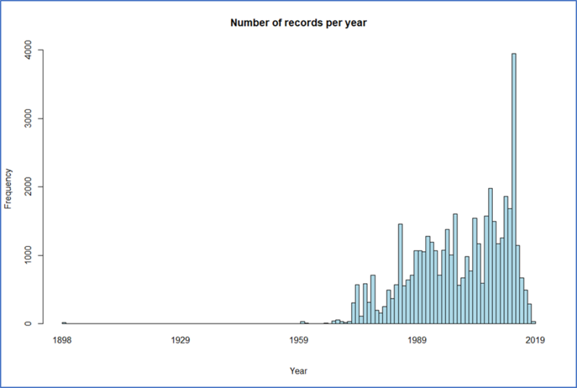
Figure 15 Age of species records from Marine Recorder used in the development and testing of predictive models.
Click for a full description
Histogram showing the age of species records from Marine Recorder used in the development and testing of predictive models. The x-axis shows the age of the records and the y-axis frequency of records. The records range from records from 1898 which are outliers to the main cluster of records ranging from 1959-2019. The number of records increases along the x-axis with most records collected between 1989 and 2019. The most records collected in a single year was 4,000 in 2014. From1989-2019, the number of records is typically between 500 and 2,000. Number of records has decreased from 2014.
Environmental data limitations
Limitations in data availability and data resolution also reduce confidence in the species models to an unknown extent. Many environmental variables are correlated and identifying causal relationships is challenging. Further limitations are due to uncertainties inherent in matching species records to environmental data collected separately and at different times.
The lack of consistent recording and reporting of environmental variables in survey data meant that environmental variables associated with survey data were extracted from separate datasets. The presence of species in habitats which were considered not to be suitable, for example, sedimentary infauna recorded as present in rock habitats, may either reflect issues with survey data and coverage or point to the existence of habitat mosaics or small areas of suitable habitat within broadly unsuitable habitat. Given the low numbers of records and surveys these could conceivably bias results.
Predictions of abundance and biomass
Abundance and biomass mapping was undertaken in order to provide context in cases where small species present in high abundances could bias interpretation. This is clearly demonstrated by the maps for Hydrobia spp. where some of the highest abundances (1,000-10,000 individuals) were predicted for this species. However, biomass based on this abundance was low due to the small size of individuals (0.002-0.005g, Obolewski & Piesik, 2010).
Biomass estimates that could be used consistently across the prey species were relatively difficult to find, as studies report weights using a variety of measures (shell free, ashed, wet weights, specific body tissues etc.) and the assessment typically is based on single references, many of which were not from the UK. Wet weight with shell was selected as the measure for biomass maps. As organisms grow their weight increases so that the weight of an organism will also depend on size and age. M. edulis and M. arenaria are longer lived than other prey species and have a greater range in length and hence weight. For these species, the biomass value selected was chosen to represent an individual that was small enough to be consumed as prey by seaduck. These values may under or overestimate the available prey biomass, but without information on size classes present at a site this is not possible to determine. The indicative biomass values were provided to support interpretation, but they should not be interpreted as indicating the actual level of biomass of prey available for seaduck.
Biotope mapping and species records
The core records for the UK Marine Habitat Classification form the basis of the biotope associations used to underpin the biotope mapping approach. However, it should be recognised that the Habitat Classification is a tool to describe and manage marine habitats. The number of records and the fidelity of species to biotopes varies considerably and caution should be exercised in interpreting associations and outputs. The hierarchy focusses only on species recorded in more than 20% of the core biotope records for a given biotope and therefore does not include every single species that may be found in a recognisable biotope or habitat Species may also be absent from habitats in which they are considered characterising, as few species are present in 100% of core biotope records.
Functional group approach
The seaduck prey identified in the review by BTO (Woodward and Humphreys, unpublished) was frequently not identified to species or genus level within the literature and these higher taxon levels cannot be matched or used to identify a refined group of biotopes within the UK Marine Habitat Classification System. Therefore, these prey categories cannot be utilised to identify potential foraging habitats based on named taxa.
As seaduck may have some dietary flexibility and be able to consume a wide range of prey items consideration was given as to whether a functional group approach based on higher taxon groupings (e.g. bivalves, small gastropods, etc.) may provide a more useful level at which to model and map prey resources. The project has not been able to fully consider the evidence available to such approaches and its validity. However, a review of unpublished trait data (compiled by H. Tillin), found that for many bivalves and gastropods (the only groups tested), readily available data sources are limited and information on habitat preferences was restricted to a few species. At the class level (Bivalvia, Gastropoda), the habitats in which members are present varies widely and that even at the genus level there may be a wide range of habitats utilised, suggesting that ability to discriminate between habitats may be limited. Collection of trait information is time-consuming and information not be readily available for many species.
Conclusions and Recommendations
This project trialled two approaches, predictive species modelling and biotope analysis, to predict the occurrence of suitable habitats for 12 principal prey species of selected seaduck. The approaches were applied to two target SPAs, the Moray Firth and the Outer Firth of Forth and St Andrews Bay Complex.
The predictive maps derived from species modelling and biotope analysis were evaluated using evidence on habitat suitability for principal prey species, collated by the project, and mapped environmental information for both of the target SPAs. The mapped distribution of the seaduck within the two target SPAs was used to assess the overlap between favourable areas for seaduck (based on their abundance and/or density) and habitats predicted to be suitable for the principal prey species.
The approach demonstrated the strengths and weaknesses of both approaches and the value of undertaking both. Many of the limitations identified and discussed by the project are considerations for all species distribution modelling work and are not unique to this study. Predictive modelling performance was limited by the overlap of species presence and absence records across modelled environmental gradients and by limited data to produce training and testing datasets. Biotope-based approaches, based on analysis of the UK Marine Habitat Classification, describe the habitat envelope of species. However, the strength of characterising species association with biotopes (the likelihood that they occur consistently within the biotope) varies. Also, some species have not been assigned to biotopes as these are based on the most common and consistently occurring species.
From the evidence review, a number of factors that underpin the development of predictive species models were identified. In general, species models typically perform better where these are limited to geographic area and where data is collected by synoptic sampling strategies that are designed to support the model work and supported by expert knowledge of local conditions, patterns and trends in species distribution and the factors that underlie these. Species models with high predictive power, as identified in the evidence review, were often the result of extensive contemporaneous surveys within areas with good spatial coverage of suitable and unsuitable habitats and appropriately resolved (spatial or temporal) evidence of key environmental or other factors influencing the population.
General ecological understanding of population dynamics allows important causal factors to be identified, including those that indirectly affect principal prey species population dynamics. Where a site has been monitored over time, trends can also become apparent. Expert insight into local patterns of species distribution and underlying factors also increase either model performance and/or interpretation. The identified evidence gaps for testing models could be addressed by targeted surveys of prey species using appropriate sampling methods. However, undertaking extensive surveys to ground-truth and map prey species and habitats is resource intensive. Although many of the principal prey species occur within the intertidal they also are present in deeper subtidal areas and therefore require vessel-based sampling. This precludes collection of prey species data through citizen science projects and student project work. In addition, many of the prey species live within sediments and are not readily sampled by drop-down camera but require the collection and processing of grab samples. Other work within SPAs, such as condition monitoring and baseline surveys undertaken ahead of human activities to support impact assessments, may provide opportunities to collect samples.
Focussed sampling in restricted areas to assess prey species distribution could be informed by predictive modelling and biotope mapping and evidence for site use by seaduck. Information on seaduck foraging areas may be easier to collect and could use remote survey methods such as camera surveys or mobilise sampling resources through citizen science or university research projects for students (Graham and Thompson, 2023).
In summary, the current project has shown the value of predictive species modelling and biotope analysis and mapping approaches to support identification of suitable habitats for seaduck prey. The approaches have discriminated between areas of suitable and unsuitable habitat within the target SPAs. However, outputs should be interpreted carefully alongside information on the ecology of prey species and observed seaduck habitat preferences.
References
Ansell, A.D., 1975. Seasonal changes in biochemical composition of the bivalve Astarte montagui in the Clyde Sea area. Marine Biology, 29(3), pp.235-243.
Ansell, A.D. and Lagardère, F., 1980. Observations on the biology of Donax trunculus and D. vittatus at Ile d'Oleron (French Atlantic Coast). Marine Biology, 57(4), pp.287-300.
Armonies, W. and Reise, K. 2003. Empty habitat in coastal sediments for populations of macrozoobenthos. Helgoland Marine Research, 56(4), 279-287.
Boldina, I. and Beninger, P.G. 2013. Fine-scale spatial structure of the exploited infaunal bivalve Cerastoderma edule on the French Atlantic coast. Journal of Sea Research, 76, 193-200.
Bustnes, J.O., Asheim, M., Bjørn, T.H., Gabrielsen, H. and Systad, G.H., 2000. The diet of Steller's Eiders wintering in Varangerfjord, northern Norway. The Wilson Journal of Ornithology, 112(1), 8-13.
Connor, D.W., Brazier, D.P., Hill, T.O. and Northen, K.O., 1997. Marine biotope classification for Britain and Ireland. Joint Nature Conservation Review, Peterborough, UK.
Connor, D.W., Allen, J.H., Golding, N., Howell, K.L., Lieberknecht, L.M., Northen, K.O. and Reker, J.B., 2004. The Marine Habitat Classification for Britain and Ireland. Version 04.05.
Cross, M.E., Lynch, S., Whitaker, A., O'Riordan, R.M. and Culloty, S.C., 2012. The reproductive biology of the softshell clam, Mya arenaria, in Ireland, and the possible impacts of climate variability. Journal of Marine Biology.
Darr, A., Gogina, M. and Zettler, M.L., 2014. Detecting hot-spots of bivalve biomass in the south-western Baltic Sea. Journal of Marine Systems, 134, 69-80.
Diederich, S., 2005. Differential recruitment of introduced Pacific oysters and native mussels at the North Sea coast: coexistence possible? Journal of Sea Research, 53 (4), 269-281.
Fenchel, T., 1975. Factors determining the distribution patterns of mud snails (Hydrobiidae). Oecologia, 20(1), 1-17.
Fox, A.D., 2003. Diet and habitat use of Scoters Melanitta in the Western Palearctic – a brief overview. Wildfowl, 54: 163-182.
Graham, J, and Thompson, K. 2023. Approaches to monitoring wintering waterfowl in Marine Protected Areas – Moray Firth pilot study winter 2019/20 NatureScot Research Report No. 1281
Hiscock, K. 1985. Littoral and sublittoral monitoring in the Isles of Scilly. September 22nd to 29th, 1984. Nature Conservancy Council, Peterborough, CSD Report, no. 562. Field Studies Council Oil Pollution Research Unit, Pembroke.
Hughes, B., Stewart, B., Brown, M.J. & Hearn, R.D. 1997. Studies of Common Scoter Melanitta nigra killed during the Sea Empress Oil Spill. Report to Countryside Council for Wales.
JNCC, 2015. The Marine Habitat Classification for Britain and Ireland Version 15.03. [12/11/20].
JNCC, 2016. Defining SPA boundaries at sea.
Kraan, C., van der Meer, J., Dekinga, A. and Piersma, T. 2009. Patchiness of macrobenthic invertebrates in homogenized intertidal habitats: hidden spatial structure at a landscape scale. Marine Ecology Progress Series, 383, 211-224.
Lewis, J.R. 1964. The Ecology of Rocky Shores. London: English Universities Press.
Mashnin, A., 2017. Size-weight structure and growth of Mytilus edulis L. in littoral zone of the White, Barents and Norwegian Seas (Master's thesis, UiT The Arctic University of Norway).
Obolewski, K. and Piesik, Z., 2010. Distribution and the role of Hydrobiidae on the middle Pomeranian (Darłowo-Władysławowo). Baltic Coastal Zone, 10, pp.2006-10.
Oppel, S., Meirinho, A., Ramírez, I., Gardner, B., O’Connell, A. F., Miller, P. I., & Louzao, M. 2012. Comparison of five modelling techniques to predict the spatial distribution and abundance of seabirds. Biological Conservation, 156, 94–104.
Parry, M.E.V. 2015. Guidance on Assigning Benthic Biotopes using EUNIS or the Marine Habitat Classification of Britain and Ireland, JNCC report No. 546, JNCC, Peterborough, ISSN 0963-8091
Patterson, D. 2021. Roosting behaviour of Common Scoters off Dornoch in the Moray Firth. Scottish Birds, 41:2, 121-125.
Patterson, D., Mitchell, C. and Tanner, D. 2022. Spring seaducks at Portmahomack, Moray Firth. Highland Bird Report 2021 Scottish Ornithologists’ Club, Highland Branch.
Reise, K., Herre, E., & Sturm, M. 1994. Biomass and abundance of macrofauna in intertidal sediments of Königshafen in the northern Wadden Sea. Helgoländer Meeresuntersuchungen, 48(2–3), 201–215.
Rodwell, J.S. (ed.) 1995. British Plant Communities. Volume 4. Aquatic communities, swamps and tall-herb fens. Cambridge University Press.
Rueda, J.L. and Smaal, A.C., 2004. Variation of the physiological energetics of the bivalve Spisula subtruncata (da Costa, 1778) within an annual cycle. Journal of Experimental Marine Biology and Ecology, 301(2), pp.141-157.
Rueda, J.L., Smaal, A.C. and Scholten, H., 2005. A growth model of the cockle (Cerastoderma edule L.) tested in the Oosterschelde estuary (The Netherlands). Journal of Sea Research, 54(4), pp.276-298.
Sardá, R., Pinedo, S. and Martin, D., 1999. Seasonal dynamics of macroinfaunal key species inhabiting shallow soft-bottoms in the Bay of Blanes (NW Mediterranean). Acta Oecologica, 20(4), 315-326.
Sotheran, I., Thompson, K., Benson, A., Boblin, E. and Nelson, E. (unpublished). Predictive mapping of supporting seabed habitats for inshore wintering waterfowl within marine proposed Special Protection Areas in Scotland. Report to Scottish Natural Heritage.
Tulp, I., Craeymeersch, J., Leopold, M., van Damme, C., Fey, F. and Verdaat, H., 2010. The role of the invasive bivalve Ensis directus as food source for fish and birds in the Dutch coastal zone. Estuarine, Coastal and Shelf Science, 90(3), 116-128.
Whitton, T.A., Jenkins, S.R., Richardson, C.A. and Hiddink, J.G. 2015. Changes in small scale spatial structure of cockle Cerastoderma edule (L.) post-larvae. Journal of Experimental Marine Biology and Ecology, 468, 1-10.
Willems, W. 2010. Habitat suitability models for the analysis and prediction of macrobenthos in the North Sea (Doctoral dissertation, Ghent University).
Wiseman, H.M., 2010. Quantifying the Ecosystem Role of a Suspension and a Facultative Deposit Feeding Bivalve in the New River Estuary, NC: with Responses to Changes in Nutrient and Sediment Inputs.
Woodward, I.D. & Humphreys, E. M. (unpublished). Inshore wintering waterfowl in marine proposed Special Protection Areas (pSPAs): - literature review of dietary and habitat preferences and foraging constraints (Report to Scottish Natural Heritage; Project Reference 017164)
Abbreviations
AUC: area under curve
BTO: British Trust for Ornithology
BODC: British Oceanographic Data Centre
cm: centimetre
cm/s: centimetres (cm) per second
DASSH: the Archive for Marine Species and Habitats
DEM: depth elevation model
EMODNET: European Marine Observation and Data Network
EUNIS: European Nature Information System
GAM: generalised additive model
GeMS: Geodatabase of Marine Features in Scotland
g: grams
g/m2: grams (g) per square meter (g/m2)
JNCC: Joint Nature Conservation Committee
km: kilometre
MarLIN: Marine Life Information Network
MLWS: Mean Low Water Springs
m: metre
m2: square metre
mm: millimetre
MR: Marine Recorder
MSBIAS: Marine Species of the British Isles and Adjacent Seas
MSFD: Marine Strategy Framework Directive
NBN: National Biodiversity Network
OFFSABC: Outer Firth of Forth and St Andrews Bay Complex SPA
ppt: parts per thousand (a measure of salinity),
PSU: practical salinity units
SACFOR: species abundance scale, S = Superabundant, A = Abundant,
C = Common, F = Frequent, O = Occasional, R = Rare
SAC: Special Area of Conservation
SPA: Special Protection Area
spp.: species pluralis (taxonomy), (see glossary)
SSSI: Site of Special Scientific Interest
STR: Supplementary Technical Report
WoRMS: World Register of Marine Species
‰: parts per thousand (a measure of salinity in supplementary technical report)
µm (in supplementary technical report referring to median grain size) micrometre or micron (see glossary)
Glossary
Area Under Curve (AUC): a measure of the performance of a model at correctly distinguishing between classes. For the current study, the AUC tests the ability of the model to correctly predict the presence and absence of principal prey species. The higher the AUC value the better the model performance.
Biotope: a biotope is defined as “the habitat together with its recurring associated community of species, operating together at a particular scale” (Connor et al., 1997).
Generalised additive model: in statistics, a generalised additive model (GAM) is a generalised linear model in which the linear response variable depends linearly on unknown smooth functions of some predictor variables
Inshore Wintering Waterfowl: species of divers, grebes and seaduck that winter in notable numbers in inshore waters (within 12 nautical miles of the coast).
Littoral: the area of the shore that is occupied by marine organisms which are adapted to or need alternating exposure to air and wetting by submersion, splash or spray. On rocky shores, the upper limit is marked by the top of the Littorina /Verrucaria belt and the lower limit by the top of the laminarian zone (Lewis, 1964). It is divided into separate subzones, particularly marked on hard substrata.
Marine Protected Area: defined geographical areas of the marine environment established and managed to achieve long-term nature conservation and sustainable use.
marine Special Protection Area: a type of MPA classified to protect bird species of European importance and regularly occurring migratory birds.
PSU: practical salinity units, refers to salinity defined in terms of its electrical conductivity relative to a prescribed standard. Other measures of salinity include parts per thousand (abbreviated as ppt or ‰)
ppt: parts per thousand (ppt) is a ratio often used to refer to the concentration of solutes in solutions, such as salts in water (i.e. salinity)
species pluralis (taxonomy): used after the genus name, when the actual species name cannot or need not or is not specified. The plural form of the abbreviation sp., it indicates "several species”.
Sublittoral: the zone exposed to air only at its upper limit by the lowest spring tides, although almost continuous wave action on extremely exposed coasts may extend the upper limit high into the intertidal region. The sublittoral extends from the upper limit of the large kelps and includes, for practical purposes in nearshore areas, all depths below the littoral. Various subzones are recognised (based on Hiscock, 1985.)
µm (in supplementary technical report referring to median grain size) micrometre (international spelling as used by the International Bureau of Weights and Measures, also commonly known as a micron, is an SI derived unit of length equalling one millionth of a metre (or one thousandth of a millimetre, 0.001 mm
Supplementary Technical Report
Please contact [email protected] if you would like to view the Supplementary Technical Report - Mapping principal prey resources of wintering seaducks within two marine Special Protection Areas in Scotland.


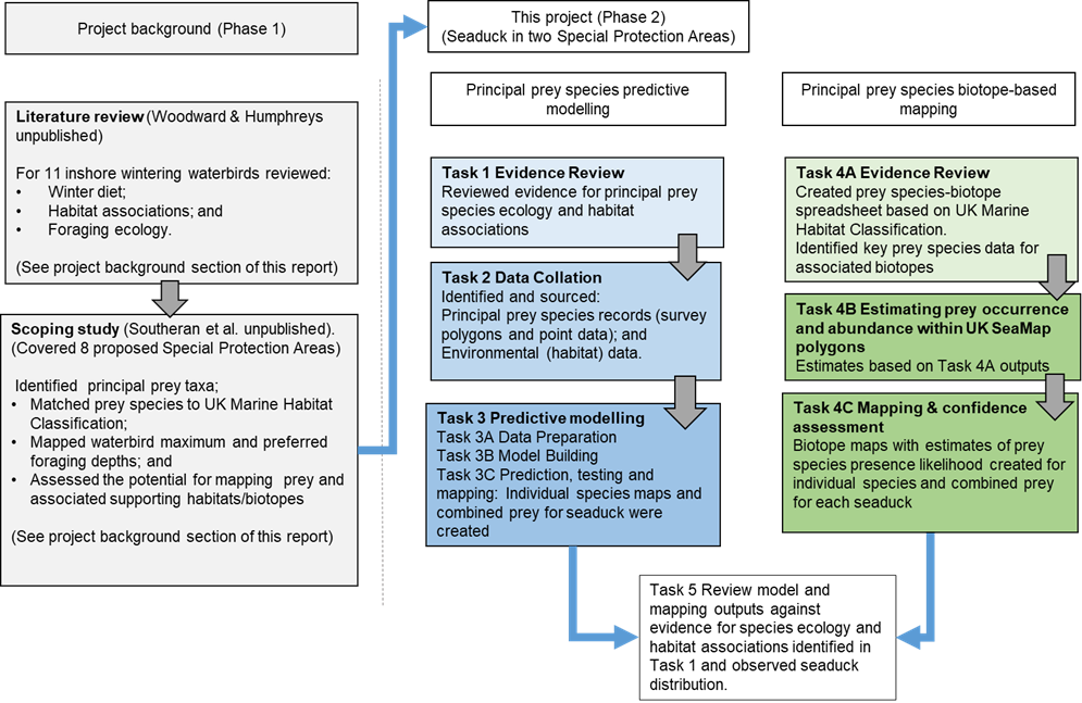
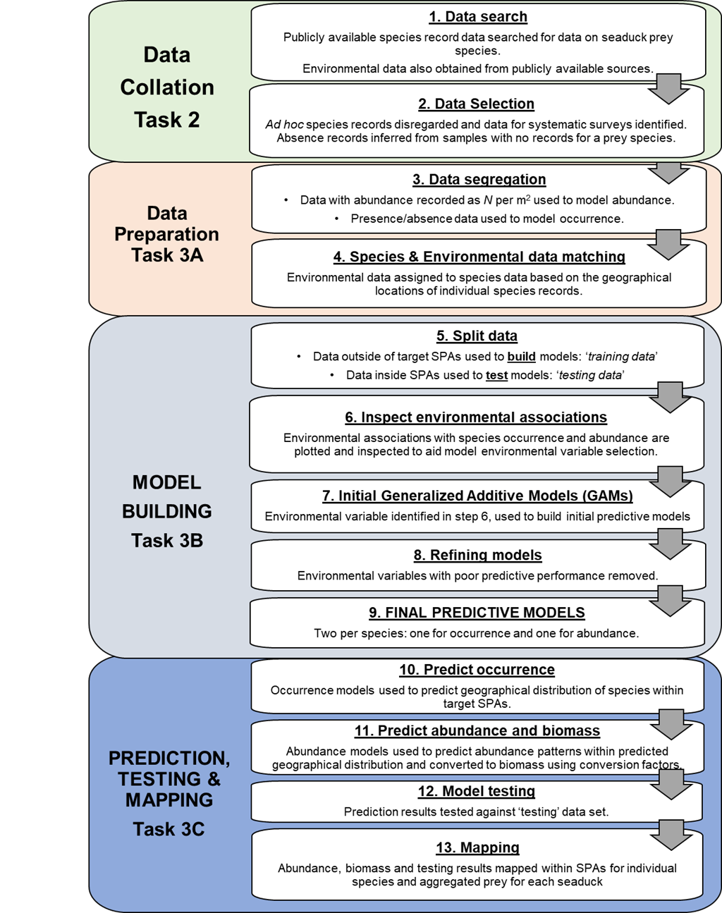
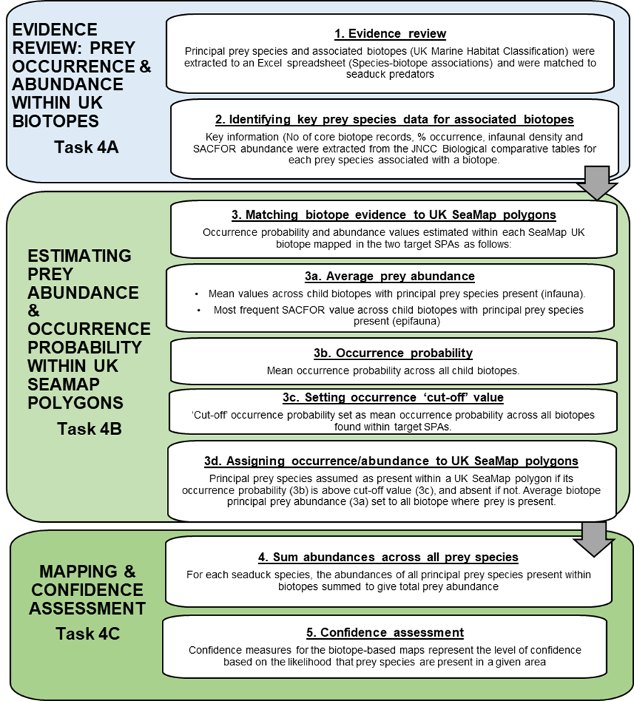
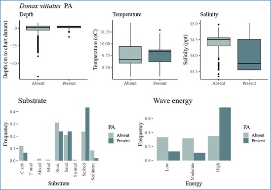