NatureScot Research Report 1399 - Assessment of recovery from dredge impacts in Loch Carron on biogenic habitats formed by Limaria hians
Published: 2026
Authors: Harries, D.B., Moore, C.G., Lyndon, A.R. and Tulbure, K.
Cite as: Harries, D.B., Moore, C.G., Lyndon, A.R. and Tulbure, K. Assessment of recovery from dredge impacts in Loch Carron on biogenic habitats formed by Limaria hians. NatureScot Research Report 1399.
Contents
- Keywords
- Background
- Main findings
- 1. Introduction
- 2. Methods
-
3. Results
- 3.1 Site relocation
- 3.2 Visual appearance
- 3.3 In situ quadrat survey of control and treatment transects (% cover of Limaria nest)
- 3.4 In situ quadrat survey of control and treatment transects (Limaria nest thickness)
- 3.5 In situ quadrat survey of control and treatment transects (binary metrics, Tables 1 and 2)
- 3.6 Quadrat clearances of control and track transects
- 3.7 Macrofaunal core samples at control and treatment transects
- 3.8 Granulometric samples from control and track transects.
- 4. Discussion
Keywords
Limaria hians; flame shells; benthic disturbance; fishing
Background
This report presents findings of a field survey of Loch Carron in 2021. The main objective of the survey was to re-assess sites initially surveyed in 2017 following damage to the Limaria hians beds in outer Loch Carron by scallop dredging (Moore et al., 2018). Three dredge impact sites were surveyed in 2017. These sites were revisited in 2021 and resurveyed employing the methodologies applied in 2017. The primary aim was to assess and quantify any recovery of this biogenic habitat from the original dredge disturbance.
Main findings
- The Limaria beds in the impacted dredge track areas at the three monitoring sites appear to have undergone a complete recovery between 2017 and 2021.
- In 2017 disturbance to the byssal nest material in the dredge track areas was visibly obvious. By 2021 the dredge track and control areas were visually indistinguishable at sites M1 and M2.
- Site M3 showed some clear differences between track and control areas in 2021. This was however attributable to pre-existing substrate differences and was unrelated to the dredge impact.
- The overall cover of Limaria nest was not markedly reduced by the dredge impact but increase of cover occurred on the dredge track area of sites M1 and M2 between 2017 and 2021.
- Features indicating disturbance, such as dead Limaria shells and exposed live Limaria tended to be more frequent on the dredge track sites than on the controls in 2017 but did not differ between track and control in 2021.
- Features indicating absence of disturbance, such as well-defined nest/sediment mosaic with clear edges tended to be more frequent on the control sites than on the dredge track sites in 2017 but did not differ between track and control in 2021.
- The abundance of Limaria in dredge track and control samples in 2021 was not significantly different.
- The size of Limaria in dredge track and control samples in 2021 was not significantly different.
- Size distribution of Limaria in the 2021 dredge track samples indicates high survival rates following the dredge impact and rapid recolonisation of the area.
- Macrofaunal cores from 2021 showed no differences in community composition between dredge track and control sites at M1 and M2.
- Recovery potential of Limaria beds from physical disturbance may vary widely depending on the reproductive health of the bed and the extent and intensity of the disturbance.
1. Introduction
In 2017, observations of dredge impacts on Limaria hians beds in Loch Carron triggered a number of impact surveys and the designation of the site as an MPA. One component of the survey work was the establishment of survey stations to facilitate the monitoring of possible recovery of the Limaria bed from dredge damage. Full details of this work are provided in Moore et al., 2018.
Prior studies of disturbance impacts and subsequent recovery of Limaria from such disturbance are limited. There are existing accounts which give evidence of impacts on Limaria beds attributed to mobile benthic fishing gear. In most instances the impacts appear persistent or were not subject to continued monitoring. Examples of such accounts include those of Hall-Spencer and Moore (2000a, b) which document long term persistent impacts on Limaria beds in the Clyde Sea area as a consequence of scallop dredging.
A further relevant study is that of Trigg and Moore 2009. This involved experimental removal of Limaria nest material from 0.25 m2 plots of seabed with subsequent periodic monitoring of recovery over a 12-month period. The study suggested a very slow rate of recovery of the nest material. It was estimated that recovery at the observed rates would take over a century to restore an area impacted by a typical set of Newhaven scallop dredges.
2. Methods
The methods employed in 2021 followed those used in 2017. Full details are provided in Moore et al., 2018 but are additionally summarised here for clarity.
2.1 Overview of sampling strategy
Potential sites for monitoring stations were identified from drop-down video surveys conducted in the area soon after the initial reports of dredge impacts in 2017. The main criteria for selection of monitoring stations were that a well-defined visible dredge track should be present within a well-developed Limaria bed (i.e., ‘pristine’ Limaria beds should lie to either side of the dredge track and the track should have clearly defined boundaries). The rationale for this was that it would provide high confidence that a well-developed Limaria bed was present prior to the 2017 dredge event and that the seabed in the impacted track could be directly compared to adjacent unimpacted Limaria beds where environmental conditions were likely to be similar to the impacted track. Meeting these criteria proved challenging because dredge marks were often not well-defined and, in many areas, it was by no means certain if a Limaria bed had been present prior to the dredging.
Potential sites were identified on the drop-down video footage and inspected by a dive team in 2017 to select those which best met the criteria. Three sites were selected (M1, M2 & M3) all of which were near the mouth of Loch Carron in the vicinity of Sgeir Bhuidhe. Locations are shown in the maps below (Figures 1 and 2) and coordinates are provided in Annex 1 (Table 1.2).
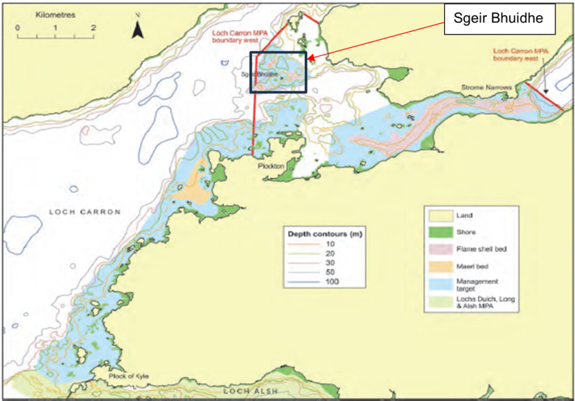
Figure 1. – Map indicating location of dredge track monitoring sites in the general context of Loch Carron (adapted from Moore et al., 2018).
Click for a full description
Map shows the northern part of Loch Alsh on its southern margin and extends to just beyond the northern extent of the Loch Carron MPA. Land areas are indicated in yellow. The outer part of Loch Carron is shown running southwest to northeast in the western half of the map. The inner part of Loch Carron extends eastwards from this in the northeastern quarter of the map. The outer boundary of the MPA is indicated by a red line where the inner part of Loch Carron joins the outer part. The Sgeir Bhuidhe dredge track monitoring area lies just within the MPA on the eastern side of the MPA boundary. It is indicated by a box with black outline.
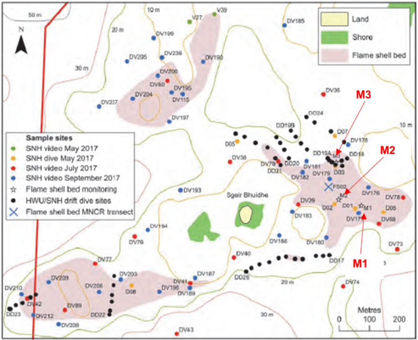
Figure 2. – Map indicating location of dredge track monitoring sites in relation to Sgeir Bhuidhe (adapted from Moore et al., 2018).
Click for a full description
Map shows the seabed in the general vicinity of the small island of Sgeir Bhuidhe. Locations of 3 known Limaria beds are indicated (northwest, west southwest and east of Sgeir Bhuidhe respectively). The dredge track monitoring sites (M1, M2 & M3) are located within the Limaria bed which lies east of Sgeir Bhuidhe.
At each of the three sites, two transects were established. The first (‘track’) was established in the centre of the dredge track and aligned with the main axis of the dredge track. The second (‘control’) was established on the neighbouring ‘pristine’ Limaria bed. It was placed in the same alignment as the track transect and within 20 m of the dredge track margin. Each transect was 10 m in length and was marked with road-pins. Additionally, the margin of the dredge track was marked with road pins in areas where it was sufficiently clear.
A series of 20 blocks of 1 m2 were established along the length of each transect (one series on the left and the other on the right). Within each block, a 0.25 m2 quadrat was placed in a pre-determined, randomly allocated position. A series of metrics were established as potential measures of the condition of the Limaria bed (see Moore et al., 2018 for details). These metrics were recorded from each quadrat in situ by a diving surveyor and photographs were taken of each quadrat. Additionally, video footage and stills photographs were taken to document the area, covering both ‘track’ and ‘control’ transects as well as the dredge track boundary.
In 2021, the methodology described above was repeated with the addition of two further elements. Firstly, the population structure and abundance of Limaria was assessed. Nest material was cleared from three 0.25 m2 quadrats at the control transect and treatment transect at all three of the dredge track sites. Live Limaria were picked out from the nest material on the deck of the boat, counted and shell length measured with digital callipers before returning the live animals to the seabed. Secondly, sediment type and infauna were assessed. Four replicate 10 cm diameter, 20 cm length macrofauna cores were collected at the control transect and track transect at all three of the dredge track sites. An additional granulometric core was also collected at each location.
Macrofaunal cores were sieved on a 0.5 mm mesh and preserved in borax buffered 10% formaldehyde. The samples were processed by Fugro GB Marine Limited. All biota were enumerated and identified to the highest practicable taxonomic resolution. A voucher collection was retained for submission to National Museums Scotland.
Granulometric samples were rinsed to eliminate salt and dried to constant weight before rehydrating and soaking in sodium hexametaphosphate. Samples were subsequently wet sieved on a 63 µm mesh and again dried to constant weight. The sievings were passed through a sieve stack with mesh sizes at half phi intervals using a mechanical sieve shaker running for 15 minutes.
2.2 Data assessment
In situ quadrat data included 2 numeric metrics and 8 binary metrics. The numeric metrics were each assessed by means of a 3 way Aligned Rank Transform ANOVA (site, year, treatment). The binary metrics were assessed using Fisher’s exact tests with comparisons made between corresponding treatments and between corresponding survey years.
For the quadrat clearances the Limaria abundance data did not meet assumptions for parametric tests and were assessed by means of a 2 way Aligned Rank Transform ANOVA (site, treatment). The Limaria size data met parametric assumptions and were assessed by means of a 2 way parametric ANOVA (site, treatment).
Macrofaunal core data were scrutinised and potentially overlapping identification categories eliminated. PRIMER was used to derive the univariate community indices of total taxa (S), total abundance (N), Pielou Evenness (J) and Shannon Weiner Diversity (H). Total taxa (S) data did not meet assumptions for parametric tests and were assessed by means of a 2 way Aligned Rank Transform ANOVA (site, treatment). The remaining indices (N, J and H) met parametric assumptions and were assessed by means of a 2 way parametric ANOVA (site, treatment). Similarity of community composition was assessed by means of non-metric multidimensional scaling (MDS) on log transformed data using the Bray-Curtis similarity coefficient. Additional analyses were also done using raw untransformed data which yielded similar results so are not presented in this report.
Granulometric samples were not replicated so statistical testing of differences is not viable. The raw data of weight of grain size fractions were converted to weight percentages and a range of granulometric parameters were derived. These encompassed median grain size, sorting coefficient (quartile deviation) and weight percentages of sediment grades within the Wentworth classification.
3. Results
3.1 Site relocation
Relocation posed some logistical challenges, but all three sites were successfully relocated. Two dives were typically required to relocate all permanent markers and deploy tapes and lines required for the repeat survey. All marker pegs were identified at M1 & M2 providing a very high degree of confidence in the spatial accuracy of the repeat survey. The marker at the end of the M3 treatment transect was missing and a tape was laid along the prescribed bearing to cover this transect. All other M3 markers were located. The distal end of the M3 treatment transect could potentially be misplaced 2 to 3 m from the 2017 placement but there is a very high degree of confidence in the spatial accuracy of the repeat survey elsewhere at M3.
3.2 Visual appearance
In 2017, the sites were selected because the path of the dredge track was visibly clearly distinct from the surrounding Limaria bed. By 2021, this visible distinction was no longer apparent at any of the three monitoring stations. Without the presence of the tagged road pins it would have been impossible to determine the location of the former dredge track.
In 2017 site M1 control was a clear mosaic with a high percentage cover of Limaria nest with well-defined edges. The track area also had a high cover of Limaria nest but this was visibly flattened, disaggregated and diffuse (Figure 3).
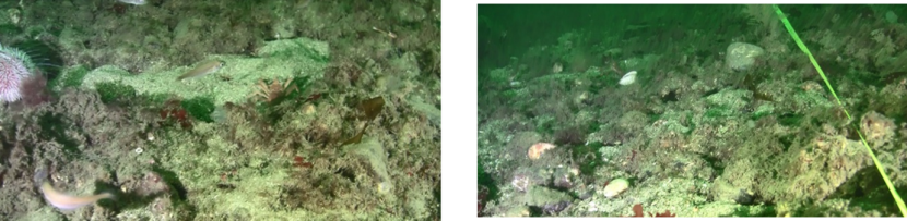
Figure 3. – Representative video screen grabs from site M1 in 2017. The control site is on the left and the track site on the right.
Click for a full description
The image of the control site shows a well-defined Limaria mosaic. The image of the track site shows diffuse Limara nest material and exposed pebbles.
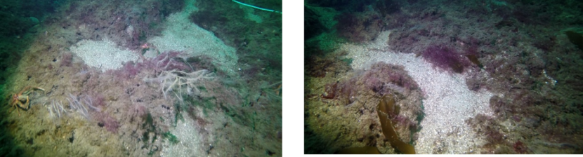
Figure 4. – Representative video screen grabs from site M1 in 2021. The control site is on the left and the track site on the right.
Click for a full description
Both images show a well-defined Limaria mosaic.
In 2021 site M1 control and track had a clear mosaic with a high percentage cover of Limaria nest with well-defined edges. The two areas were visually indistinguishable and this is apparent from both the video footage and from stills photography (Figure 4).
During the 2017 survey an attempt was made to mark the margin of the dredge track with road pins. The margin was found not to be entirely clearly defined, but divers were able to distinguish where the disrupted dredged area merged into the area of intact Limaria nests and mark the margin with pegs. In 2021 the pegs were relocated, and divers were unable to recognise a visible margin. The general area now consisted of a homogenous and continuous mosaic. The differences are not readily apparent on video screen grabs because a wider overview of the seabed is necessary to distinguish such differences (Figure 5).
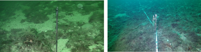
Figure 5. – Representative video screen grabs from site M1 track boundary. The image on the left is from 2017 and that on the right from 2021.
Click for a full description
The image from 2017 shows a higher proportion of open sand patches whereas the image from 2021 shows more continuous cover of Limara nest material.
The account of observations from site M2 are generally similar to those made at site M1. In 2017 site M2 control was a clear mosaic with a high percentage cover of Limaria nest with well-defined edges. The track area also had a high cover of Limaria nest but this was visibly flattened, disaggregated and diffuse (Figure 6).
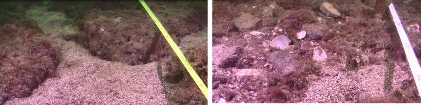
Figure 6. – Representative video screen grabs from site M2 in 2017. The control site is on the left and the track site on the right.
Click for a full description
The image of the control site shows a well-defined Limaria mosaic. The image of the track site shows diffuse Limara nest material and broken Limaria shells.
In 2021 site M2 control and track had a clear mosaic with a high percentage cover of Limaria nest with well-defined edges. The nest coverage appears slightly greater in the track than the control but the two areas were essentially visually indistinguishable and this is apparent from both the video footage and from stills photography (Figure 7).
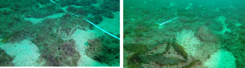
Figure 7. – Representative video screen grabs from site M2 in 2021. The control site is on the left and the track site on the right.
Click for a full description
Both images show a well-defined Limaria mosaic.
The edge of the M2 dredge track marked in 2017 was perhaps marginally better defined than that seen at M1 but was nevertheless rather indistinct. Divers were able to take a wider view and distinguish the disrupted nest material from the neighbouring mosaic of intact nests. In 2021 no such distinction was apparent. A well-developed nest mosaic was present over the entire area surrounding the boundary markers (Figure 8).
Figure 8. – Representative video screen grabs from site M2 track boundary. The image on the left is from 2017 (disturbed area on left half of image) and that on the right from 2021.
Click for a full description
The image from 2017 shows an area (on the left of the image) of diffuse and flattened Limara nest material. The image from 2021 shows a more uniform Limara nest mosaic.
Site M3 shows some clear differences from sites M1 And M2. There are differences in sediment type between the control and track transects which are likely to be a major factor in controlling the development of the Limaria bed. The control area appears to be predominantly stoney with a significant proportion of surface pebbles whereas the track area appears predominantly sandy with relatively sparse pebbles.
In 2017 site M3 control had clear Limaria habitat but it was much less well defined and had lower surface relief than was the case at sites M1 and M2. It was visibly stoney, in contrast to the sandier area of the track transect. In the 2017 M3 track transect there were sparse patches of Limaria nest material many of which appeared visibly disrupted. (Figure 9).
In 2021 the M3 control site appeared to have considerably higher cover of Limaria nest than was the case in 2017 but it appeared to have lower surface relief than was seen at M1 and M2 and lacked the clearly defined mosaic structure seen at those locations. The 2021 M3 track site had a very different appearance to the control. It appeared a generally sandy seabed with discrete weedy clumps of Limaria nest scattered over the surface (Figure 10).
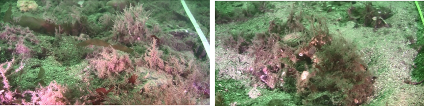
Figure 9. – Representative video screen grabs from site M3 in 2017. The control site is on the left and the track site on the right.
Click for a full description
Both images show relatively diffuse patches of Limara nest material.
Figure 10. – Representative video screen grabs from site M3 in 2021. The control site is on the left and the track site on the right.
Click for a full description
The image of the control site shows high coverage of Limaria nest material. The image of the track site shows patchy discontinuous Limara nest material.
The edge of the M3 dredge track was found to be rather poorly defined and diffuse in 2017. A boundary was however defined by the diver and marked out. When revisited in 2021 a diffuse boundary still appears to be present. This can be seen in the 2021 image in Figure 11. On the left of the image is the area of high cover of Limaria nest which corresponds to the control transect and on the right of the image is the area of large patches of open sand which corresponds to the track transect.
Figure 11. – Representative video screen grabs from site M3 track boundary. The image on the left is from 2017 and that on the right from 2021.
Click for a full description
The image from 2017 shows relatively diffuse Limara nest material with scattered pebbles. The image from 2021 shows a more extensive Limara nest mosaic.
3.3 In situ quadrat survey of control and treatment transects (% cover of Limaria nest)
Of the metrics recorded in the quadrats, the percentage cover of the turf of Limaria nest material is the most direct measure of the Limaria bed condition and these data are presented below.
At site M1 in 2017 the nest cover in the track transect was reported as reduced relative to the control transect on the basis of a parametric t-test (Moore et al., 2018). The current study (Figure 12) applied a 3-way non-parametric test and that difference is no longer significant (3-way ART ANOVA P>0.05). There is also no significant difference between track and control transects in the 2021 data. Temporal comparisons show no significant difference between survey years for the control transect but a significant increase in nest cover is present on the track transect in 2021 relative to 2017 (3-way ART ANOVA P=0.0004). Representative images from 2017 and 2021 are shown below (Figure 13).
Figure 12. – Mean percentage cover of Limaria nest cover in control and track transects at site M1 in 2017 and 2021 with standard error of the mean. Columns sharing a letter code are not significantly different.
Click for a full description
The bar graph presents 4 columns. From left to right these are: 2017 control, 2017 track, 2021 control and 2021 track. Mean percentage cover of Limaria nest appears less in 2017 track relative to the other 3 values.
Figure 13. – Representative images of site M1 track quadrats. The image on the left is from 2017 and that on the right from 2021.
Click for a full description
The image from 2017 shows relatively diffuse Limara nest material with scattered pebbles. The image from 2021 shows a more well-defined Limara nest mosaic.
At site M2 there was no significant difference between track and control in either 2017 or 2021 (Figure 14). Temporal comparisons show no significant difference between survey years for the control transect but a significant increase in nest cover is present on the track transect in 2021 relative to 2017 (3-way ART ANOVA P=0.0356). Representative images from 2017 and 2021 are shown below (Figure 15).
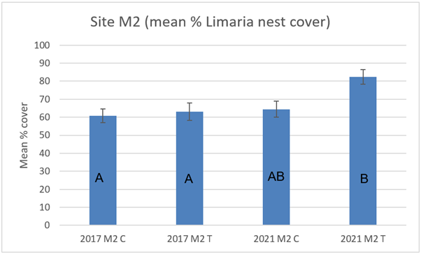
Figure 14. – Mean percentage cover of Limaria nest cover in control and track transects at site M2 in 2017 and 2021. Columns sharing a letter code are not significantly different.
Click for a full description
The bar graph presents 4 columns. From left to right these are: 2017 control, 2017 track, 2021 control and 2021 track. Mean percentage cover of Limaria nest appears slightly higher in 2021 track relative to the other 3 values.
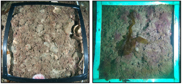
Figure 15. – Representative images of site M2 track quadrats. The image on the left is from 2017 and that on the right from 2021.
Click for a full description
The image from 2017 shows relatively diffuse Limara nest material with scattered pebbles. The image from 2021 shows more continuous Limara nest cover.
At site M3 there was significantly less nest cover in the track transect than in the control transect in both 2017 (3-way ART ANOVA P=0.0015) and 2021 (3-way ART ANOVA P<0.0001) (Figure 16). A significant (3-way ART ANOVA P<0.0001) increase in nest cover occurred on the control transect between 2017 and 2021. The corresponding temporal comparison of the track transect showed no significant difference (3-way ART ANOVA P>0.05). Representative images from 2017 and 2021 are shown below (Figure 17).
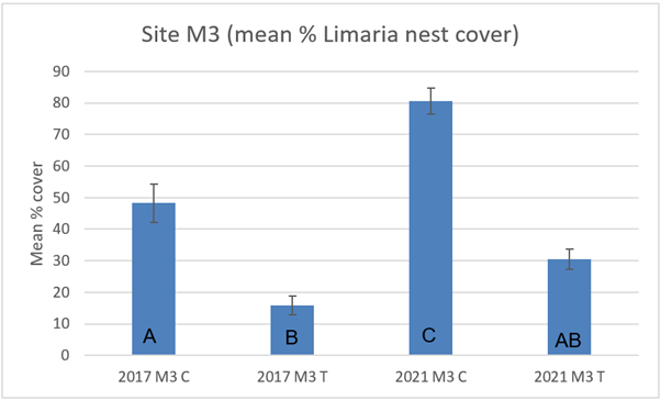
Figure 16. – Mean percentage cover of Limaria nest cover in control and track transects at site M3 in 2017 and 2021. Columns sharing a letter code are not significantly different.
Click for a full description
The bar graph presents 4 columns. From left to right these are: 2017 control, 2017 track, 2021 control and 2021 track. Mean percentage cover of Limaria nest appears slightly higher in 2021 relative to the corresponding areas in 2017. In both survey years the cover of Limaria nest is distinctly higher in the control than in the track.

Figure 17. – Representative images of site M3 track quadrats. The image on the left is from 2017 and that on the right from 2021.
Click for a full description
Both images show sparse patches of Limara nest material.
The increased nest cover in the track transects of sites M1 and M2 in 2021 relative to 2017 is consistent with recovery of the bed. The pattern at site M3 is less clear with increases in nest cover of the control transect between 2017 and 2021 but not in the track.
3.4 In situ quadrat survey of control and treatment transects (Limaria nest thickness)
At site M1 nest thickness at the control transect in 2017 was significantly higher compared to the track transect and also to the 2021 control transect (3-way ART ANOVA P<0.0001) (Figure 18). Control and track transect were not significantly different in 2021 and there was no significant change in the track transect between 2017 to 2021 (3-way ART ANOVA P>0.05).
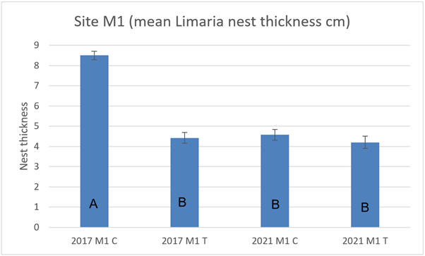
Figure 18. – Mean Limaria nest thickness in control and track transects at site M1 in 2017 and 2021. Columns sharing a letter code are not significantly different.
Click for a full description
The bar graph presents 4 columns. From left to right these are: 2017 control, 2017 track, 2021 control and 2021 track. Mean Limaria nest thickness is distinctly higher in 2017 control relative to the other 3 values.
At site M2 nest thickness was not significantly different between track and control in either 2017 or 2021 (Figure 19), but nest thickness in both cases was significantly (3-way ART ANOVA P<0.001) reduced in 2021 relative to 2017.
Figure 19. – Mean Limaria nest thickness in control and track transects at site M2 in 2017 and 2021. Columns sharing a letter code are not significantly different.
Click for a full description
The bar graph presents 4 columns. From left to right these are: 2017 control, 2017 track, 2021 control and 2021 track. Mean Limaria nest thickness appears slightly higher in 2017 than in 2021.
At site M3 nest thickness at the control transect in 2017 was significantly (3-way ART ANOVA P<0.0001) lower compared to the track transect and also to the 2021 control transect (Figure 20). Control and track transect were not significantly different in 2021 and there was no significant change in the track transect between 2017 to 2021.
Figure 20. – Mean Limaria nest thickness in control and track transects at site M3 in 2017 and 2021. Columns sharing a letter code are not significantly different.
Click for a full description
The bar graph presents 4 columns. From left to right these are: 2017 control, 2017 track, 2021 control and 2021 track. Mean Limaria nest thickness is distinctly lower in 2017 control relative to the other 3 values.
Overall, there is no consistent change apparent in terms of nest thickness differences between control and track or change over time.
3.5 In situ quadrat survey of control and treatment transects (binary metrics, Tables 1 and 2)
In 2017 the track transect of site M1 showed some indications of disturbance in terms of reduction in quadrat frequency (relative to the control) of clearly defined nest mosaic with well-defined boundaries and in terms of increased frequency of exposed Limaria and dead shells. In 2021 the increased frequency of exposed Limaria and dead shells was no longer apparent. However, the data still indicated a reduction in frequency of the clearly defined nest mosaic with well-defined boundaries in the track transect. A re-examination of the photo quadrats shows that in 2017 the mosaic was indeed partly degraded and flattened. However, in 2021 the reason that some of the track quadrats recorded absence of mosaic and clear boundaries was that those quadrats fell on areas of 100 % nest cover and hence no mosaic or boundaries were present. So, the apparent indication of mosaic disturbance is an artefact in the 2021 data and occurred due to increased coverage of nest material.
Similarly, the 2017 track transect of site M2 showed some indications of disturbance in terms of reduction in frequency (relative to the control) of clearly defined nest mosaic with well-defined boundaries and in terms of increased frequency of dead Limaria shells. In 2021 none of these disturbance metrics differed between control and track.
In 2017 the track transect of site M3 showed a lower frequency (relative to the control) of well-defined mosaic, continuous patches of turf and visible Limaria gallery apertures. The only remaining difference between track and control in 2021 was in the frequency of well-defined nest mosaic. However, the trend is reversed relative to that of 2017 with a greater frequency of nest mosaic recorded in the track transect. Again, this appears to be an artefact. In the 2021 control transect a greater number of quadrats fell on areas of 100 % Limaria cover and hence the presence of a mosaic was not recorded. In both 2017 and 2021 the control transect was on a well-developed Limaria bed whereas the track transect was on a relatively bare sandy area with sparse nest patches. The clear increase in nest cover on the control between 2017 and 2021 has caused the difference in this metric despite it being visually apparent that nest cover has also increased on the track transect.
| Parameter | M1C | M1T | p | M2C | M2T | p | M3C | M3T | p |
|---|---|---|---|---|---|---|---|---|---|
| Byssal material present (# quadrats) | 20 | 20 | 1.000 | 20 | 20 | 1.000 | 20 | 18 | 0.244 |
| Continuous turf present locally (# quadrats) | 20 | 20 | 1.000 | 20 | 20 | 1.000 | 19 | 14 | 0.046 |
| Byssus overtops stones (# quadrats) | 20 | 20 | 1.000 | 20 | 19 | 0.500 | 20 | 16 | 0.053 |
| Turf/clean sand mosaic (# quadrats) | 20 | 15 | 0.024 | 20 | 14 | 0.010 | 19 | 4 | <0.001 |
| Gallery apertures seen (# quadrats) | 20 | 20 | 1.000 | 20 | 20 | 1.000 | 20 | 11 | <0.001 |
| Limaria seen (# quadrats) | 0 | 7 | 0.008 | 1 | 3 | 0.605 | 0 | 1 | 1.000 |
| Dead Limaria shells (# quadrats) | 1 | 10 | 0.001 | 2 | 15 | <0.001 | 2 | 3 | 0.500 |
| Sharp turf boundary present (# quadrats) | 20 | 13 | 0.004 | 20 | 10 | <0.001 | 5 | 3 | 0.347 |
| Parameter | M1C | M1T | p | M2C | M2T | p | M3C | M3T | p |
|---|---|---|---|---|---|---|---|---|---|
| Byssal material present (# quadrats) | 20 | 20 | 1.000 | 20 | 20 | 1.000 | 20 | 20 | 1.000 |
| Continuous turf present locally (# quadrats) | 20 | 20 | 1.000 | 20 | 20 | 1.000 | 20 | 19 | 0.500 |
| Byssus overtops stones (# quadrats) | 20 | 20 | 1.000 | 20 | 20 | 1.000 | 20 | 17 | 0.115 |
| Turf/clean sand mosaic (# quadrats) | 18 | 10 | 0.007 | 19 | 17 | 0.302 | 12 | 19 | 0.010 |
| Gallery apertures seen (# quadrats) | 20 | 20 | 1.000 | 20 | 20 | 1.000 | 20 | 16 | 0.053 |
| Limaria seen (# quadrats) | 0 | 1 | 1.000 | 1 | 0 | 1.000 | 0 | 0 | 1.000 |
| Dead Limaria shells (# quadrats) | 2 | 3 | 0.500 | 6 | 7 | 0.500 | 0 | 0 | 1.000 |
| Sharp turf boundary present (# quadrats) | 20 | 10 | <0.001 | 20 | 20 | 1.000 | 0 | 0 | 1.000 |
A temporal comparison of the binary quadrat data (Tables 3, 4 and 5) confirms the general pattern of recovery seen above (Tables 1 and 2). At site M1 there were no significant changes to any of the parameters on the control transect from 2017 to 2021. On the track transect the frequency of exposed Limaria and of dead shells was lower in 2021 than 2017.
| - | M1C | M1C | M1C | M1T | M1T | M1T |
|---|---|---|---|---|---|---|
| Parameter | 2017 | 2021 | p | 2017 | 2021 | p |
| Byssal material present (# quadrats) | 20 | 20 | 1.000 | 20 | 20 | 1.000 |
| Continuous turf present locally (# quadrats) | 20 | 20 | 1.000 | 20 | 20 | 1.000 |
| Byssus overtops stones (# quadrats) | 20 | 20 | 1.000 | 20 | 20 | 1.000 |
| Turf/clean sand mosaic (# quadrats) | 20 | 18 | 0.244 | 15 | 10 | 0.071 |
| Gallery apertures seen (# quadrats) | 20 | 20 | 1.000 | 20 | 20 | 1.000 |
| Limaria seen (# quadrats) | 0 | 0 | 1.000 | 7 | 1 | 0.044 |
| Dead Limaria shells (# quadrats) | 1 | 2 | 0.500 | 10 | 3 | 0.020 |
| Sharp turf boundary present (# quadrats) | 20 | 20 | 1.000 | 13 | 10 | 0.262 |
Similarly, at site M2 there were no significant changes to any of the parameters on the control transect from 2017 to 2021. On the track transect the frequency of dead Limaria shells was lower in 2021 than 2017 and the frequency of clear nest boundaries was higher in 2021.
| - | M2C | M2C | M2C | M2T | M2T | M2T |
|---|---|---|---|---|---|---|
| Parameter | 2017 | 2021 | p | 2017 | 2021 | p |
| Byssal material present (# quadrats) | 20 | 20 | 1.000 | 20 | 20 | 1.000 |
| Continuous turf present locally (# quadrats) | 20 | 20 | 1.000 | 20 | 20 | 1.000 |
| Byssus overtops stones (# quadrats) | 20 | 20 | 1.000 | 19 | 20 | 0.500 |
| Turf/clean sand mosaic (# quadrats) | 20 | 19 | 0.500 | 14 | 17 | 0.225 |
| Gallery apertures seen (# quadrats) | 20 | 20 | 1.000 | 20 | 20 | 1.000 |
| Limaria seen (# quadrats) | 1 | 1 | 1.000 | 3 | 0 | 0.231 |
| Dead Limaria shells (# quadrats) | 2 | 6 | 0.118 | 15 | 7 | 0.012 |
| Sharp turf boundary present (# quadrats) | 20 | 20 | 1.000 | 10 | 20 | <0.001 |
At site M3 there was a decrease in frequency of clearly defined nest mosaic with well-defined boundaries between 2017 to 2021 on the control transect. As stated above, this is attributable to the increase in nest cover on the control transect resulting on more quadrats falling on continuous turf with no mosaic or boundaries apparent. On the track transect there is a significant increase in the frequency of areas of continuous turf from 2017 to 2021 and a corresponding increase in the frequency of well-developed nest mosaic. This supports the observation of visibly higher nest cover on the track in 2021 as compared to 2017.
| - | M3C | M3C | M3C | M3T | M3T | M3T |
|---|---|---|---|---|---|---|
| Parameter | 2017 | 2021 | p | 2017 | 2021 | p |
| Byssal material present (# quadrats) | 20 | 20 | 1.000 | 18 | 20 | 0.244 |
| Continuous turf present locally (# quadrats) | 19 | 20 | 0.500 | 14 | 19 | 0.046 |
| Byssus overtops stones (# quadrats) | 20 | 20 | 1.000 | 16 | 17 | 0.500 |
| Turf/clean sand mosaic (# quadrats) | 19 | 12 | 0.010 | 4 | 19 | <0.001 |
| Gallery apertures seen (# quadrats) | 20 | 20 | 1.000 | 11 | 16 | 0.088 |
| Limaria seen (# quadrats) | 0 | 0 | 1.000 | 1 | 0 | 1.000 |
| Dead Limaria shells (# quadrats) | 2 | 0 | 0.244 | 3 | 0 | 0.115 |
| Sharp turf boundary present (# quadrats) | 5 | 0 | 0.024 | 3 | 0 | 0.115 |
The pattern of differences seen in the binary quadrat data are consistent with the picture of Limaria bed recovery. Metrics indicative of disturbance show some differences between track and control in 2017 but genuine differences are absent in 2021. This is confirmed by temporal comparisons of transects which show no genuine changes on the control transect from 2017 to 2021 whereas disturbance metrics tend to have significantly reduced frequency on the 2021 track transects as compared to the corresponding 2017 transects.
3.6 Quadrat clearances of control and track transects
Quadrat clearances were conducted in 2021 and allow assessment of Limaria abundance and population structure. Temporal comparison with 2017 is not possible because corresponding samples were not collected at that time, but we are able to assess for differences between track and control in 2021.
The abundance of Limaria in the cleared quadrats (Figure 21) was not significantly different between control and track transect at any of the 3 monitoring sites (ART ANOVA P>0.05 for ‘treatment’). There was however significantly lower abundance of Limaria at site M3 than at each of the other two sites (ART ANOVA P<0.05 for ‘site’).
Figure 21. – Mean Limaria abundance in the cleared quadrats from control and track transects in 2021.
Click for a full description
The bar graph presents 6 columns. From left to right these are: M1 control, M1 track, M2 control, M2 track, M3 control and M3 track. Mean Limaria abundance appears lower at M3 relative to the other 2 sites.
The mean size of Limaria (Figure 22) was not significantly different between control and track transect at any of the 3 monitoring sites (2-way ANOVA P>0.05 for ‘treatment’). The mean size at M3 appears slightly smaller than at each of the other two sites. However, the difference is not statistically significant (2-way ANOVA P>0.05 for ‘site’).
Figure 22. – Mean Limaria size in the cleared quadrats from control and track transects in 2021. No significant differences were detected.
Click for a full description
The bar graph presents 6 columns. From left to right these are: M1 control, M1 track, M2 control, M2 track, M3 control and M3 track. Mean Limaria size shows some variability, but differences are not statistically significant.
3.7 Macrofaunal core samples at control and treatment transects
3.7.1 Univariate community indices
The total number of taxa (S) present in the macrofaunal cores (Figure 23) was not significantly different between control and track samples at any of the 3 sites and there were no significant differences between the 3 sites in 2021 (ART ANOVA P >0.05). Temporal comparison with 2017 is not possible because corresponding samples were not collected at that time, but we are able to assess for differences between track and control in 2021.
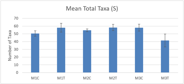
Figure 23. – Mean total number of taxa present in macrofaunal cores (10 cm diameter) from control and track transects in 2021. No significant differences were detected.
Click for a full description
The bar graph presents 6 columns. From left to right these are: M1 control, M1 track, M2 control, M2 track, M3 control and M3 track. Mean total number of taxa shows some variability, but differences are not statistically significant.
The total individual specimens (N) present in the macrofaunal cores (Figure 24) was not significantly different between control and track samples at any of the 3 sites (2-way ANOVA ‘treatment’ P>0.05) in 2021. There was a significant difference between sites with lower numbers recorded at M3 relative to M2 (2-way ANOVA ‘site’ P<0.01).
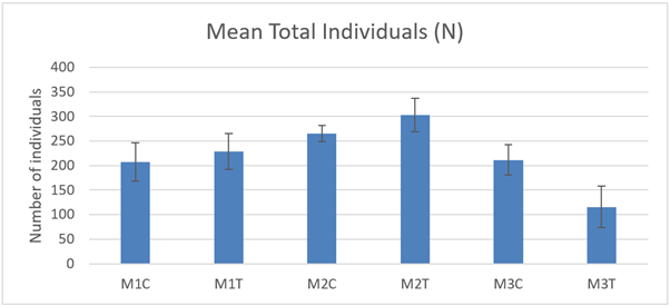
Figure 24. – Mean total number of individual specimens present in macrofaunal cores (10 cm diameter) from control and track transects in 2021.
Click for a full description
The bar graph presents 6 columns. From left to right these are: M1 control, M1 track, M2 control, M2 track, M3 control and M3 track. Mean total number of individual specimens appear slightly lower at M3 relative to M2.
Pielou Evenness (J) was not significantly different between control and track macrofaunal core samples (Figure 25) at any of the 3 sites and there were no significant differences between sites (2-way ANOVA P >0.05) in 2021.
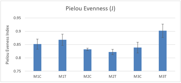
Figure 25. – Mean Pielou Evenness (J) in macrofaunal cores (10 cm diameter) from control and track transects in 2021. No significant differences were detected.
Click for a full description
The bar graph presents 6 columns. From left to right these are: M1 control, M1 track, M2 control, M2 track, M3 control and M3 track. Mean Pielou Evenness (J) shows some variability, but differences are not statistically significant.
Shannon Wiener diversity (H) was not significantly different between control and track macrofaunal core samples (Figure 26) at any of the 3 sites and there were no significant differences between sites (2-way ANOVA P >0.05) in 2021.
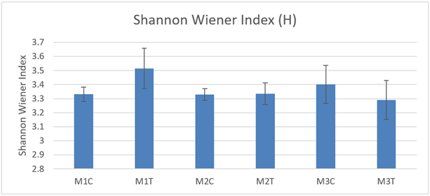
Figure 26. – Mean Shannon Wiener diversity (H) in macrofaunal cores (10 cm diameter) from control and track transects in 2021. No significant differences were detected.
Click for a full description
The bar graph presents 6 columns. From left to right these are: M1 control, M1 track, M2 control, M2 track, M3 control and M3 track. Mean Shannon Wiener diversity (H) shows some variability, but differences are not statistically significant.
3.7.2 Multivariate community analysis
Two alternative datasets were assessed by multivariate statistical tests. One where all poorly resolved identifications were pooled at a higher taxonomic level and the other where poorly resolved identifications were removed from the dataset. Both approaches yielded consistent outputs. The data presented below is derived from the dataset where poorly resolved identifications were removed.
The MDS for site M1 (Figure 27) shows clearly overlapping similarity between control and track samples. This is confirmed by ANOSIM which indicates no evidence of a difference in community composition between control and track samples (R=0, Significance = 48.6%).
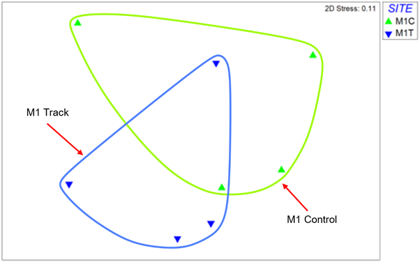
Figure 27 – MDS plot of macrofauna core samples from site M1. Data is log transformed and Bray-Curtis similarity coefficient was applied.
Click for a full description
The MDS plot shows 4 replicate samples from the control site as green triangle symbols, and these are encircled by a green line. The 4 replicates from the track site are shown by blue triangle symbols encircled by a blue line. There is clear overlap between the control and track replicates indicating no consistent difference in community composition.
Similarly, the MDS for site M2 (Figure 28) shows clearly overlapping similarity between control and track samples. This is confirmed by ANOSIM which indicates no evidence of a difference in community composition between control and track samples (R=0.073, Significance = 37.1%).
The MDS for site M3 (Figure 29) shows some separation between control and track samples. The separation is largely a consequence of two distinctly impoverished samples from the track (cores 1 and 4). ANOSIM indicates some evidence of a difference in community composition between control and track samples (R=0.427, Significance = 2.9%). However, the low R value does not provide convincing evidence of a clear difference given the high variability in the composition of the track samples.
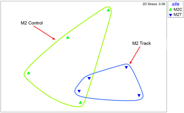
Figure 28 – MDS plot of macrofauna core samples from site M2. Data is log transformed and Bray-Curtis similarity coefficient was applied.
Click for a full description
The MDS plot shows 4 replicate samples from the control site as green triangle symbols, and these are encircled by a green line. The 4 replicates from the track site are shown by blue triangle symbols encircled by a blue line. There is clear overlap between the control and track replicates indicating no consistent difference in community composition.
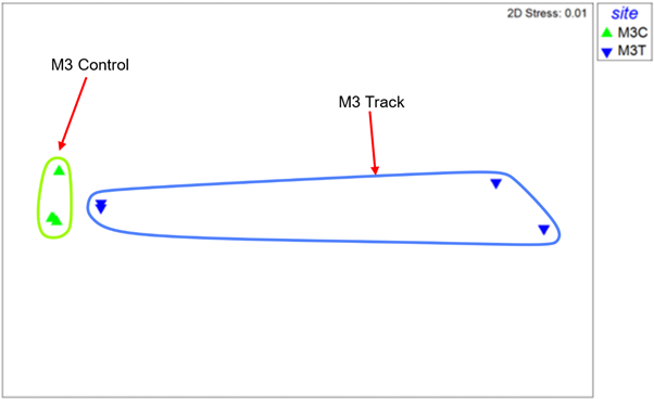
Figure 29 – MDS plot of macrofauna core samples from site M3. Data is log transformed and Bray-Curtis similarity coefficient was applied.
Click for a full description
The MDS plot shows 4 replicate samples from the control site as green triangle symbols, and these are encircled by a green line. The 4 replicates from the track site are shown by blue triangle symbols encircled by a blue line. The track replicates show some differences from the control but they are highly variable in composition and show no clear consistent differences from the control replicates.
3.8 Granulometric samples from control and track transects.
Granulometric samples were collected in 2021 and enable subjective comparisons to be made between the track and control transects at each of the sites. It is not considered likely that the dredge disturbance will have created a measurable change in granulometry. The purpose of the comparison is to assess if granulometric differences might mirror any observed biological differences between track and control. Samples were not replicated so no statistical comparisons are possible. Selected granulometric parameters are presented in Table 6. The percentage gravel (>4 mm) content is cited for the entire sample whereas the remaining sediment parameters are based on the data with the gravel (>4 mm) content excluded. The rationale for this approach is that the chance occurrence of one or two larger pebbles within the sample has a disproportionate effect on the other granulometric parameters.
Whole sample | M1C | M1T | M2C | M2T | M3C | M3T |
|---|---|---|---|---|---|---|
% Gravel (>4 mm) | 15.1 | 16.4 | 8.8 | 23.3 | 31.1 | 6.8 |
- | - | - | - | - | - | - |
Sample excluding gravel (>4 mm) | M1C | M1T | M2C | M2T | M3C | M3T |
Median grain size (mm) | 0.33 | 0.44 | 0.5 | 0.41 | 0.33 | 0.52 |
Sorting coefficient (quartile deviation in phi) | 1.15 | 1.15 | 1.18 | 1.23 | 1.28 | 1.00 |
% Silt & Clay (<63 µm) | 12.9 | 12.9 | 9.4 | 15.0 | 14.2 | 6.3 |
The proportion of coarser particles (gravel, small pebbles and shell fragments) is likely to be of biological relevance because such particles provide the necessary anchor points for the byssal threads used for Limaria nest building. Gravel (>4 mm) content (Figure 30) is consistent between track and control at site M1, it is higher at M2T than at M2C and is lower at M3T than at M3C. The greatest disparity is that at site M3. It should be recognised that surface gravel and pebbles are often patchily distributed so there is likely to be considerable variance between the relatively small granulometric cores. However, the low proportion of surface pebbles at M3T relative to M3C is visibly apparent in the underwater imagery from the site.
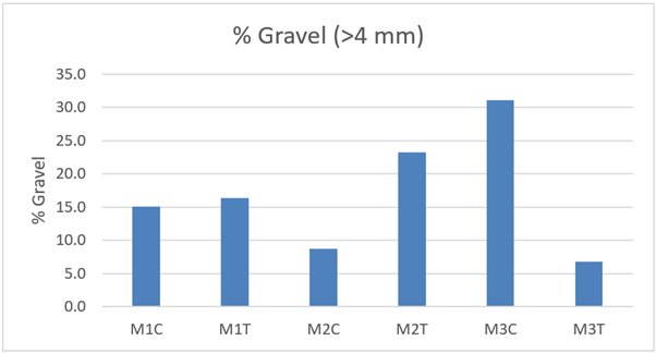
Figure 30 – Percentage gravel (>4 mm) from control and track transects in 2021. Samples were not replicated so no statistical comparisons are possible.
Click for a full description
The bar graph presents 6 columns. From left to right these are: M1 control, M1 track, M2 control, M2 track, M3 control and M3 track. Percentage gravel (>4 mm) is similar in control and track at M1. It is slightly higher in track than control at M2 and is markedly higher in control than track at M3.
The proportion of silt / clay is also often of biological relevance because of its effect on the physical properties of the sediment. Silt / clay content (Figure 31) is consistent between track and control at site M1, it is higher at M2T than at M2C and is lower at M3T than at M3C. The greatest disparity is that at site M3.
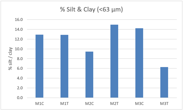
Figure 31 – Percentage silt / clay (<63 µm) content from control and track transects in 2021. Samples were not replicated so no statistical comparisons are possible.
Click for a full description
The bar graph presents 6 columns. From left to right these are: M1 control, M1 track, M2 control, M2 track, M3 control and M3 track. Percentage silt / clay (<63 µm) is similar in control and track at M1. It is slightly higher in track than control at M2 and is slightly higher in control than track at M3.
In terms of median grain size the differences between track and control samples at sites M1 and M2 are relatively minor (~100 µm) disparity. There is a slightly greater difference (~200 µm) between track and control samples at site M3 (Table 6).
In terms of sorting coefficients the track and control samples at sites M1 and M2 are very similar to each other. There is a somewhat larger difference between track and control samples at site M3 with better sorted sediment at site M3T.
The general picture is of poorly sorted medium to coarse slightly muddy sand with a significant gravel component. Site M3T shows some granulometric differences with a lower proportion of both gravel and silt / clay. The consequence of this is that it is rather better sorted and has slightly higher median grain size (due to reduced silt / clay).
4. Discussion
4.1 Change and recovery at the Loch Carron monitoring sites
The overall outcome of this investigation is that the dredge track damage which was apparent at the three monitoring sites in 2017 was no longer apparent in 2021. This suggests that the Limaria beds impacted by the dredge had recovered within the 4-year period between these surveys.
In 2017 the dredge damage was visibly apparent in the track area of all three monitoring sites. In all three, the track area was visibly distinct from the control area. The damage did not manifest as mass removal of Limaria nest but consisted of visible nest disruption, disaggregation and flattening. In 2021 there was no longer any well-defined visible difference between the track and control areas at sites M1 and M2. A clear visible difference between track and control areas was still apparent for site M3 in 2021 but this difference is attributable to substrate differences between the track and control areas rather than indicating any legacy of the dredge damage.
The 2017 survey quantified dredge damage by means of in situ data recorded from a series of replicate quadrats within control and track areas at each of the three sites. A series of metrics were devised as indicators of physical disturbance of Limaria beds and these metrics were recorded within each quadrat. In 2021 this procedure was repeated and additionally samples were collected for laboratory assessment. These consisted of macrofaunal core samples, granulometric samples and quadrat clearances to assess Limaria size and population density.
The metric of percentage cover of Limaria nest might seem intuitively to be most closely related to physical disturbance impacts. However, the anticipated reduction of nest cover in the 2017 dredge tracks was not apparent as a consistent trend. This is due to the fact that the passage of the dredge did not result in mass removal of nest material but instead left a trail of broken and disaggregated nest material on the seabed, so percentage cover of nest was not necessarily significantly reduced.
At site M1 the nest cover in the track in 2017 was lower than in the control but the difference was not significant. By 2021 the cover in the track had significantly increased and was similar to that recorded in the 2017 and 2021 control sites. This pattern of change is consistent with recovery from the dredge impact. The nest cover at site M2 followed a similar pattern of no difference between track and control in either survey year but a significant increase in cover in the track transect between 2017 and 2021. In fact, the 2021 nest cover in the M2 track appeared higher (but not significantly so) than in the control. It is possible that at this site there was a preexisting difference whereby the track area was more suitable than the control area for supporting dense nest development.
Site M3 was recognised in 2017 to be sub optimal as a monitoring site and it was suggested that it may be in a transition zone near the Limaria bed margin (Moore et al., 2018). The key issue with the site is that there are clear pre-existing substrate differences between the control and track areas. On-site imagery shows a much higher proportion of surface pebbles in the control area. In the track area there are extensive patches of open sandy sediment with few surface pebbles. Limaria require anchorage points for the byssal threads used for nest construction, and pebbles and shell fragments commonly serve as such anchorage points. In the absence of sufficient anchorage points it is likely that nest establishment will be curtailed resulting in reduced coverage of Limaria nest material. The 2021 granulometric data also support the visual assessment of substrate type. The sample from the M3 track contained distinctly less coarse (>4 mm) and fine (<63 µm) sediment fractions than seen at all other sites. It is probable that the reduced amount of coarse particles is a consequence of local physical or geological processes (i.e. simply a sandy patch on the seabed). The reduced proportion of fine particles may have a biological cause in that the absence of pebbles prevents the development of biological turfs which would entrap and accumulate fine particles.
The nest cover at M3 was distinctly different in nature to that seen at M1 and M2. At M1 and M2 the Limaria formed a well-defined mosaic of raised nest material interspersed with sand patches. The nest cover at site M3 control had relatively low surface relief and lacked the clear mosaic structure seen at sites M1 and M2. Nest cover at M3 track consisted of relatively sparse isolated patches separated by areas of sand. In 2017 there was visible damage in the M3 track area and nest cover was significantly lower than in the control area. However, it is likely that the substrate difference was the main factor behind this difference in nest cover. In 2021 this substrate driven difference in nest cover between track and control remained apparent. By 2021 nest cover had increased in both areas of M3 and this increase was significant for the control area. We are unable to explain this temporal increase in nest cover at the M3 control area. Although visible evidence of disturbance was not noted on the M3 control in 2017 it cannot be discounted that it had been impacted and the subsequent increase in nest cover represents recovery from this impact.
It was assumed that Limaria nest thickness would provide a useful metric for assessing nest disturbance. This proved not to be the case and nest thickness showed no clear and consistent trends in relation to disturbance. The subjective impression of the surveyors was that the nest thickness showed considerable variation and was difficult to measure with confidence. This may have resulted in some inter-surveyor variability in the data. Additionally, dredge disturbance does not necessarily have a consistent effect on nest thickness. The piling up of displaced nest material may cause localised thickening in some patches within the dredge track while adjacent patches may become thinner due to removal of nest material. Consequently, the interpretation of the nest thickness data is problematic and inconclusive so is not considered further.
The remaining metrics recorded in the quadrats included some indicative of disturbance (e.g. live Limaria exposed on the sediment surface and presence of dead Limaria shells on the surface) and some indicative of the absence of disturbance (e.g. presence of a well-defined mosaic with clear boundaries at nest margins). The overall picture from these metrics supports the observation of physical damage in 2017 and subsequent recovery by 2021. For the M1 2017 data the metrics mentioned above all show the expected trend of increased disturbance levels on the track transect. Site M2 was similar although a difference in live exposed Limaria was not noted (this might be expected to be transient due to predation on exposed Limaria). In 2021 none of the metrics differed between track and control at site M2 and the only differences at site M1 were due to an artefact (nest expansion resulting in no mosaic or boundaries present in individual quadrats). Temporal changes at the M1 and M2 sites show a corresponding pattern. No changes were apparent on the control areas of either site between 2017 to 2021. However, the track areas showed changes indicative of recovery from disturbance with less exposed or dead Limaria seen in 2021 on M1 and less dead Limaria and more pronounced nest boundaries seen in 2021 on M2.
Changes at site M3 are complicated by the substrate differences mentioned above. However, the data do reflect a similar pattern to that seen at M1 and M2. The M3 track in 2017 showed lower frequency of byssus turf, defined nest mosaic and visible gallery apertures when compared to the control. In 2021 the only difference between track and control was a lower frequency of mosaic records in the control. This was determined to be a consequence of the marked expansion of nest coverage in the M3 control resulting in more quadrats landing on continuous nest cover rather than mosaics. This also shows in the temporal comparison with the only changes in the control site between 2017 to 2021 being attributable to the same cause. The temporal comparison of the M3 track site shows evidence of recovery with increased frequency of byssus turf and nest mosaic in 2021 relative to 2017.
The remaining data from the project derive from samples collected in 2021. No corresponding sampling was conducted in 2017, so temporal comparisons are not possible. However, comparisons can be drawn between track and control samples to assess if there is evidence for any continued differences which might be attributable to the dredge disturbance.
The abundance of Limaria in the cleared quadrats (n = 3 per site) showed no significant difference between track and control at any of the sites in 2021. This is consistent with the pattern of recovery shown in the data discussed above. The abundance of Limaria at site M3 was lower than at M1 and M2 and this is consistent with the noted substrate differences at M3 and the observation that it was located near the bed margin. It should be noted that the clearances were selectively taken from dense areas of nest material, so they represent a measure of Limaria abundance within the area of nest coverage rather than Limaria abundance in the area as a whole. Had clearances been taken from random positions then some would land on patches of bare sand and result in lower mean abundance and greater variance in the data. This would be particularly pronounced in areas with more sand patches such as the M3 track site.
A similar pattern is apparent for mean Limaria size with no significant difference between track and control at any of the sites in 2021. Sizes were marginally lower at site M3 but the difference is not statistically significant.
The macrofaunal core samples again parallel the general trend. For sites M1 and M2 there is no evidence of a difference between track and control in the composition of the macrofaunal communities in 2021. This holds true for comparisons based on total taxa, total abundance, indices of diversity and evenness and those based on multivariate tests of community similarities.
Site M3 is similar in terms of there being no evidence of differences between track and control in total taxa, total abundance, indices of diversity and evenness. There is however tentative evidence of differences between track and control in community composition revealed by the multivariate testing. The data show there is considerable variability in the composition of the M3 track samples with two samples in particular being very impoverished in relation to all others. This is assuredly related to the highly patchy substrate present at the M3 track and unrelated to the 2017 disturbance event. It is also notable that total abundance in the macrofauna cores from M3 was significantly lower than at sites M1 and M2. Again, this is consistent with the observation that M3 lay at the bed margin.
Hence, all the available evidence indicates a full recovery of the Limaria beds at the three monitoring sites with no detectable ongoing consequences of the 2017 dredge disturbance event. Although this is encouraging it should be acknowledged that it relates to only three study sites. It does not entirely rule out the possibility that longer term consequences may have been precipitated in other areas of the Loch Carron seabed. It should be noted, however, that analysis of dropdown video footage collected from the Sgeir Bhuidhe Limaria beds in 2023 (Moore, 2025) also revealed an indication of temporal enhancement of byssal turf development at some locations since 2017, and there was strong evidence that the bed containing the monitoring transect sites M1 – M3 had extended beyond its 2017 limits, with the development of a well-formed, sand/turf mosaic where the habitat was previously recorded as absent and where the seabed previously exhibited signs of dredge damage.
4.2 Wider implications
Limaria nest disturbance and recovery is likely to involve a number of processes. The initial disturbance event clearly disrupted nest galleries, killing or exposing at least some of the Limaria. It is known that Limaria displaced from their nests are capable of rebuilding the galleries relatively rapidly over a matter of days (Tulbure unpublished data). However, the individuals exposed on the surface following disturbance are often rapidly predated by crabs and squat lobsters (pers. obs.) so displacement is likely to often prove fatal before the protective structure of the nest can be rebuilt.
For this reason, we consider that recolonisation will be necessary to enable the full recovery of the bed from a disturbance event. A significant proportion of the population may survive within the disrupted nest fabric and succeed in the rebuilding and repair of the galleries but many may be directly killed by crushing or predated when ejected from the galleries. Recovery of the population to baseline levels will require compensating for such losses. Settlement of planktonic larvae may play a key role in this recovery but it is also possible that migration of post settlement adults from neighbouring areas may be significant. It is known that adults can relocate and colonise suitable substrates (Cook, 2016; Tulbure unpublished data) but the scale and frequency of this behaviour is unknown.
Pre-existing data on age / length relationships in Limaria (Eckford-Soper 2009, Trigg 2009) indicate that individuals of 4 years or less in age rarely exceed 30 mm in size. At the Loch Carron monitoring sites 4 years elapsed between the 2017 disturbance event and the quadrat clearance sampling conducted in 2021. Consequently, it is improbable that individuals more than 30 mm in size became established in the dredge track through post 2017 larval settlement. At each of the three monitoring sites about 40% of the individuals sampled on the track areas were greater than 30 mm in size. These then must represent survivors of the dredge impact and / or post settlement individuals which migrated into the track areas after the disturbance event. If anything, this figure of 40% is likely to be an underestimate because at least some of the individuals less than 30 mm in size may be older than 4 years. Additionally, over 80% of the individuals in the track areas were greater than 20 mm in size. The majority of animals in this size range are likely to be at least 3 years in age. This would suggest that most of the recolonisation of the dredge track probably occurred soon after the disturbance event.
The relatively rapid recovery documented at Loch Carron would appear to be at odds with the findings of the experimental study conducted at Port Appin by Trigg and Moore (2009). That study found a very slow rate of recovery which when extrapolated up to the scale of a commercial scallop dredge would indicate a recovery time of over a century. A number of factors might contribute to explaining the very different outcome observed at Loch Carron. One is the intensity of the disturbance event. In the Port Appin experiment it was assumed that the scallop dredge would strip away the entirety of the nest material. Consequently, all nest material was removed from the experimental plots, the underlying sediment was raked and larger stones removed. This constitutes a rather more intense level of disturbance than that resulting from the scallop dredge in Loch Carron where nest material was flattened and disrupted but mostly remained present on the seabed. At least some of the population of Limaria will have remained viable in Carron and the remaining byssal material will have had a stabilising effect facilitating the rebuilding of nest structures. The removal of stones in the Port Appin experimental plots may also be significant. Limaria require anchorage points for their byssal threads in order to build nests and the bare sandy patches created in the Port Appin experimental plots are likely to have provided limited anchorage points. Further factors that might explain the discrepancy between these studies include interannual variability in recruitment and possible differences in environmental ‘health’ at the two sites. It is well established that recruitment levels in many benthic invertebrates show considerable interannual variability. In some years there may be virtually no successful recruitment whereas in other years there may be mass recruitment and population explosions. It is possible that 2017 / 2018 may simply have been a high recruitment year for Limaria and 2006 / 2007 when the Port Appin study was conducted may have been a recruitment failure. A significant point to note is that in the years following the experimental study the extensive bed at Port Appin underwent a sustained and pronounced decline (Cook, 2016). This reached the stage where by 2018 the bed appeared to be virtually entirely absent (Scottish Government, 2020). The reason for the decline of the Port Appin bed is not clear but it is possible that the limited recovery seen in the 2006 experimental study was because the bed was already in decline with recruitment failures for unrelated reasons.
The reason for the discrepancy between the recovery observed in Loch Carron and the lack of recovery in the Clyde (Hall-Spencer and Moore (2000a, b) is rather more clear cut. The impacts in the Clyde were a consequence of sustained and repeated dredging whereas Carron experienced a single dredging event followed by imposition of protective measures. The case of Carron then could be regarded as a success story for prompt conservation intervention. The Limaria has recovered from the 2017 dredging event but it is probable that if repeated dredging had occurred then the Limaria bed would be degraded to a level from where recovery would not take place.
4.3 Recommendations for further work
Developing an enhanced understanding of response and recovery of biogenic habitats from fishery related disturbance is problematic. Planned field experimental work would offer the ideal approach to gaining that understanding, and it would ideally be conducted on different types of bed, use different types of fishing gear and apply different frequencies of disturbance. The obvious problem is that this would create an unacceptable level of damage to a habitat type which is known to be both uncommon and sensitive to disturbance. Scaled down experimental work can be considered, but extrapolating findings from a small-scale experiment to predict the effects of a larger scale disturbance is likely to be highly error prone.
The Carron study offered a chance opportunity to learn from an unplanned disturbance event. Such events are likely to occur again in the future. It would be prudent to consider how to react rapidly should such circumstances arise again in the future and initiate a monitoring programme in a timely fashion. This was achieved in Carron and has changed our understanding of the potential of Limaria beds to recover from physical disturbance. The use of fixed site markers to confirm accuracy of relocation was very beneficial. If coordinates alone had been used, then the findings of the work would be very questionable.
It is regrettable that no physical sampling was conducted in 2017. This decision was taken to avoid further damage to the bed. The decision was justified, but hindsight would indicate that the benefit from information gained from limited sampling would have outweighed the limited damage that the sampling would have caused. Some thought should be given to the choice of in-situ metrics to be recorded. A range of metrics were recorded at Loch Carron and given the difficulties of predicting the most useful metrics in advance, it is good policy to cover a range of options. In addition to the recording of in-situ metrics it is highly recommended that imagery (video and/or stills) is collected extensively to evaluate change directly and minimise the issues of inter surveyor variation and differences in perception of different individuals. An evaluation of the effectiveness of the different metrics collected in the study of Loch Carron is presented below (Table 7).
| Metric | Sensitivity in current study | Subjective assessment of usefulness of the metric |
|---|---|---|
| Percent cover of nest material based on estimates made in replicate quadrats. | Temporal changes in cover were detected at all 3 sites. | The metric is useful, but it should be noted that disturbance does not necessarily result in total removal of nest material and the distinction of disturbed from pristine nest material is not always clear cut. So, cover of nest material in an obviously disturbed location may not differ from that of an equivalent undisturbed location. |
| Nest thickness based on estimates made in replicate quadrats. | No consistent differences were apparent in terms of nest thickness between control and track sites or change over time. | Metric has limited usefulness. Nest thickness was highly variable and difficult to measure with consistency. Disturbance does not necessarily have a consistent effect on nest thickness. The piling up of displaced nest material may cause localised thickening in some patches while adjacent patches may become thinned. |
| Presence of byssal material within replicate quadrats. | No differences detected between track and control and no temporal change detected. | Metric is not useful because at least some byssal material is likely to remain present even within a disturbed area. |
| Presence of area of continuous turf (>10x10 cm) within replicate quadrats. | Detected a difference between control and track at one site in 2017. Detected a temporal change between 2017 to 2021 at a further site. | Metric has potential value as areas of continuous turf are less likely to remain following physical disturbance. |
| Presence of byssal material covering stones within replicate quadrats. | No differences detected between track and control and no temporal change detected. | Metric is not useful because it is difficult to assess if stones are present below the byssus mat without removing the overlying nest material. Observations indicate stones are sometimes exposed by disturbance and are more likely to be visible on the surface at disturbed sites. An improved metric might be the presence of surface stones partially or entirely detached from the byssus mat. |
| Presence of Turf/sand mosaic (clean sand patches >10x10 cm) within replicate quadrats. | Showed differences between track and control in the 2017 data as well as certain other differences in the dataset. | The metric is useful but needs to be interpreted with caution. Well defined mosaic beds might be disrupted by disturbance and result in a lower frequency of mosaics. However, some of our data showed a reduced frequency of mosaics that was attributable to expansion of nest material such that cover was more continuous and mosaics were consequently less frequently recorded. |
| Presence of gallery apertures within replicate quadrats. | A difference was detected between track and control at one site in 2017. | Metric has limited usefulness. Gallery apertures might be destroyed by disturbance but holes in the byssal mat may be created by the disturbance and are sometimes difficult to distinguish from the apertures created by the Limaria. Additionally, intact gallery apertures are not always readily visible even in undisturbed pristine beds. |
| Presence of exposed living Limaria within replicate quadrats. | More exposed Limaria recorded in the track at one site in 2017. | Metric has limited usefulness. It is certainly the case that more Limaria may become exposed on the surface of the seabed following disturbance of the byssus mat. However, observations show that once displaced from their nests they are often rapidly predated by crabs. So the exposed Limaria are likely to be rapidly removed and only provide an indicator of disturbance for a short period following the disturbance event. |
| Presence of dead Limaria shells within replicate quadrats. | An increased frequency of dead Limaria shells were recorded in the track areas of 2 sites in 2017. | Metric has potential value as disturbance events are likely to result in more dead shells on the surface and these are likely to remain present for a considerable period. However dead shells may also be present on a healthy bed and differences in frequency are not pronounced. |
| Presence of sharp turf boundary within replicate quadrats. | Showed differences between track and control at 2 sites in the 2017 data as well as certain other differences in the dataset. | The metric is useful but is related to the ‘mosaic’ metric and similarly needs to be interpreted with caution. Disturbance may disrupt the bed topography and result in a lower frequency of clear-cut boundaries. However, expansion of nest material to form a continuous cover will also result in a reduced frequency of clear-cut boundaries. |
| Limaria abundance assessed through the clearance of nest material in replicate quadrats. | No data available from 2017 and no differences detected between track and control in 2021. | This metric is the most direct and reliable measure of the abundance of Limaria. Its effectiveness at evaluating disturbance is not verified because destructive sampling was avoided in 2017. |
| Infaunal community composition assessed through collection of infaunal cores. | No data available from 2017 and no differences detected between track and control in 2021. | This metric is the most direct and reliable measure of the composition of the communities associated with Limaria beds. Its effectiveness at evaluating disturbance is not verified because destructive sampling was avoided in 2017. |
Assessing the health of a Limaria bed in terms of disturbance impacts requires a holistic approach and is difficult to capture from any single metric of condition. Visible disruption of the bed can be evident in some cases but individual metrics that indicate disturbance may not capture the full picture. The table below outlines some of the distinctions that might be expected between an undisturbed bed and one subject to physical disturbance (Table 8).
| Undisturbed | Disturbed |
|---|---|
| Variable levels of cover of nest material. | Reduced levels of nest cover in some cases although significant disturbance can occur without a measurable decrease in cover. |
| Bed topography of a relatively even undulating surface of byssus mat and / or a well-defined mosaic of raised areas of byssus mat with clearly defined edges adjacent to patches of bare sediment. | Diffuse or irregular areas of byssus mat. Often with a ‘flattened’ appearance. Mosaics are less well defined, and the edges of the nest patches are less distinctly raised and lack the sharp edges of an undisturbed mosaic. |
| Surface of byssus mat relatively free of loose pebbles, shell fragments and gravel. | Relatively more stone / shell debris loose and lying on the surface of the byssus mat. |
| Visible live Limaria rarely seen exposed on the sea bed. | Live Limaria frequently seen exposed on the seabed immediately following a disturbance event. These are normally scavenged / predated and are unlikely to be evident after a few days / hours. |
| Dead Limaria shells are infrequently seen on the sea bed. | Relatively high frequency of dead Limaria shells may persist for some time following disturbance but will progressively degrade or become buried with the passage of time. |
| Limaria abundance likely to be relatively high within the undisturbed byssus matrix. | Limaria abundance is likely to be reduced following a disturbance event but this may not be detectable in areas of lower disturbance intensity. |
| Diverse community of associated biota is likely to be present upon and within an undisturbed byssus mat. | The associated community is likely to be modified as a consequence of a disturbance event but this may not be detectable in areas of lower disturbance intensity. |
Acknowlegements
Many thanks to Bally Philp for providing the boat and good company. Thank you also to Alex Robertson-Jones and Owen Paisley for dive support at Loch Carron in 2021.
5. REFERENCES
Cook, R.L. 2016. Development of techniques for the restoration of temperate biogenic reefs. PhD thesis, Heriot-Watt University.
Eckford-Soper, L. 2009. Population structure and growth of Limaria hians (Bivalvia) from west coast Scottish Sea Lochs. MSc dissertation, Heriot-Watt University.
Hall-Spencer, J.M. and Moore, P.G. 2000a. Limaria hians (Mollusca: Limacea): a neglected reef forming keystone species. Aquatic Conservation – Marine and Freshwater Ecosystems 10, 267–277.
Hall-Spencer, J.M. and Moore, P.G. 2000b. Scallop dredging has profound long-term impacts on maerl habitats. ICES Journal of Marine Science 57, 1407–1415.
Moore, C.G. 2026. Biological analyses of underwater video from monitoring and research cruises carried out from 2021 to 2023 in the Clyde Sea, Sound of Barra, Loch Carron, Loch Eriboll and off Wester Ross. NatureScot Research Report. In press.
Moore, C.G., Harries, D.B., James, B., Cook, R.L., Saunders, G.R., Tulbure, K.W., Harbour, R.P. and Kamphausen, L. 2018. The distribution and condition of flame shell beds and other Priority Marine Features in Loch Carron Marine Protected Area and adjacent waters. Scottish Natural Heritage Research Report, no. 1038, Scottish Natural Heritage.
Scottish Government 2020. Scotland’s Marine Assessment 2020. Biogenic Habitats.
Trigg, C. 2009. Ecological Studies on the bivalve Limaria hians (Gmelin) PhD thesis, Heriot-Watt University.
Trigg, C. and Moore, C.G. 2009. Recovery of the biogenic nest habitat of Limaria hians (Mollusca: Limacea) following anthropogenic disturbance, Estuarine, coastal and shelf science, 82(2), pp. 351-356.
ANNEX 1: FLAME SHELL BED RECOVERY MONITORING TRANSECT DATA
Year | Site | Treatment | Byssal material present (Y/N) | Continuous turf present (i.e. >10x10 cm locally) Y/N | Turf cover (%) | Byssus overtops stones (Y/N) | Turf/sand mosaic (clean sand patches >10x10 cm) (Y/N) | Gallery apertures (Y/N) | Mean turf thickness (cm) | Limaria seen (Y/N) | Dead Limaria shells (Y/N) | Sharp turf boundary present (Y/N) |
|---|---|---|---|---|---|---|---|---|---|---|---|---|
2017 | M1 | C | Y | Y | 70 | Y | Y | Y | 8 | N | N | Y |
2017 | M1 | C | Y | Y | 90 | Y | Y | Y | 8 | N | N | Y |
2017 | M1 | C | Y | Y | 60 | Y | Y | Y | 8 | N | N | Y |
2017 | M1 | C | Y | Y | 80 | Y | Y | Y | 8 | N | N | Y |
2017 | M1 | C | Y | Y | 50 | Y | Y | Y | 8 | N | N | Y |
2017 | M1 | C | Y | Y | 60 | Y | Y | Y | 10 | N | N | Y |
2017 | M1 | C | Y | Y | 80 | Y | Y | Y | 10 | N | N | Y |
2017 | M1 | C | Y | Y | 70 | Y | Y | Y | 10 | N | N | Y |
2017 | M1 | C | Y | Y | 85 | Y | Y | Y | 7 | N | N | Y |
2017 | M1 | C | Y | Y | 70 | Y | Y | Y | 8 | N | N | Y |
2017 | M1 | C | Y | Y | 70 | Y | Y | Y | 10 | N | N | Y |
2017 | M1 | C | Y | Y | 50 | Y | Y | Y | 8 | N | N | Y |
2017 | M1 | C | Y | Y | 95 | Y | Y | Y | 8 | N | N | Y |
2017 | M1 | C | Y | Y | 60 | Y | Y | Y | 9 | N | Y | Y |
2017 | M1 | C | Y | Y | 80 | Y | Y | Y | 8 | N | N | Y |
2017 | M1 | C | Y | Y | 80 | Y | Y | Y | 8 | N | N | Y |
2017 | M1 | C | Y | Y | 60 | Y | Y | Y | 10 | N | N | Y |
2017 | M1 | C | Y | Y | 30 | Y | Y | Y | 8 | N | N | Y |
2017 | M1 | C | Y | Y | 50 | Y | Y | Y | 8 | N | N | Y |
2017 | M1 | C | Y | Y | 70 | Y | Y | Y | 8 | N | N | Y |
2017 | M1 | T | Y | Y | 30 | Y | N | Y | 3 | N | N | N |
2017 | M1 | T | Y | Y | 60 | Y | N | Y | 4 | Y | Y | N |
2017 | M1 | T | Y | Y | 75 | Y | N | Y | 4 | N | Y | Y |
2017 | M1 | T | Y | Y | 60 | Y | Y | Y | 4 | N | N | N |
2017 | M1 | T | Y | Y | 45 | Y | Y | Y | 4 | Y | N | Y |
2017 | M1 | T | Y | Y | 85 | Y | Y | Y | 6 | N | Y | Y |
2017 | M1 | T | Y | Y | 75 | Y | Y | Y | 7.5 | N | N | Y |
2017 | M1 | T | Y | Y | 60 | Y | Y | Y | 5 | N | N | Y |
2017 | M1 | T | Y | Y | 60 | Y | Y | Y | 5 | N | N | Y |
2017 | M1 | T | Y | Y | 20 | Y | Y | Y | 4 | N | Y | N |
2017 | M1 | T | Y | Y | 40 | Y | Y | Y | 4 | Y | Y | Y |
2017 | M1 | T | Y | Y | 90 | Y | N | Y | 4 | N | Y | N |
2017 | M1 | T | Y | Y | 75 | Y | N | Y | 4 | N | N | N |
2017 | M1 | T | Y | Y | 45 | Y | Y | Y | 6 | Y | N | Y |
2017 | M1 | T | Y | Y | 50 | Y | Y | Y | 6 | Y | Y | Y |
2017 | M1 | T | Y | Y | 30 | Y | Y | Y | 4 | N | N | Y |
2017 | M1 | T | Y | Y | 40 | Y | Y | Y | 4 | Y | Y | N |
2017 | M1 | T | Y | Y | 15 | Y | Y | Y | 4 | N | N | Y |
2017 | M1 | T | Y | Y | 10 | Y | Y | Y | 2 | Y | Y | Y |
2017 | M1 | T | Y | Y | 45 | Y | Y | Y | 4 | N | Y | Y |
2017 | M2 | C | Y | Y | 60 | Y | Y | Y | 8 | Y | N | Y |
2017 | M2 | C | Y | Y | 85 | Y | Y | Y | 7 | N | N | Y |
2017 | M2 | C | Y | Y | 50 | Y | Y | Y | 8 | N | N | Y |
2017 | M2 | C | Y | Y | 75 | Y | Y | Y | 9 | N | N | Y |
2017 | M2 | C | Y | Y | 50 | Y | Y | Y | 8 | N | N | Y |
2017 | M2 | C | Y | Y | 60 | Y | Y | Y | 10 | N | N | Y |
2017 | M2 | C | Y | Y | 50 | Y | Y | Y | 7 | N | N | Y |
2017 | M2 | C | Y | Y | 90 | Y | Y | Y | 8 | N | N | Y |
2017 | M2 | C | Y | Y | 50 | Y | Y | Y | 7 | N | N | Y |
2017 | M2 | C | Y | Y | 65 | Y | Y | Y | 8 | N | N | Y |
2017 | M2 | C | Y | Y | 75 | Y | Y | Y | 10 | N | N | Y |
2017 | M2 | C | Y | Y | 50 | Y | Y | Y | 9 | N | N | Y |
2017 | M2 | C | Y | Y | 15 | Y | Y | Y | 10 | N | N | Y |
2017 | M2 | C | Y | Y | 50 | Y | Y | Y | 8 | N | Y | Y |
2017 | M2 | C | Y | Y | 75 | Y | Y | Y | 8 | N | N | Y |
2017 | M2 | C | Y | Y | 65 | Y | Y | Y | 7 | N | N | Y |
2017 | M2 | C | Y | Y | 65 | Y | Y | Y | 8 | N | N | Y |
2017 | M2 | C | Y | Y | 70 | Y | Y | Y | 7 | N | N | Y |
2017 | M2 | C | Y | Y | 75 | Y | Y | Y | 8 | N | N | Y |
2017 | M2 | C | Y | Y | 40 | Y | Y | Y | 9 | N | Y | Y |
2017 | M2 | T | Y | Y | 50 | Y | Y | Y | 8 | N | N | Y |
2017 | M2 | T | Y | Y | 55 | Y | N | Y | 6 | N | Y | Y |
2017 | M2 | T | Y | Y | 65 | Y | Y | Y | 8 | Y | Y | N |
2017 | M2 | T | Y | Y | 60 | Y | Y | Y | 10 | Y | Y | Y |
2017 | M2 | T | Y | Y | 40 | Y | N | Y | 6 | N | Y | N |
2017 | M2 | T | Y | Y | 55 | Y | Y | Y | 10 | Y | Y | Y |
2017 | M2 | T | Y | Y | 55 | Y | N | Y | 8 | N | Y | Y |
2017 | M2 | T | Y | Y | 20 | Y | Y | Y | 10 | N | N | Y |
2017 | M2 | T | Y | Y | 65 | Y | Y | Y | 8 | N | Y | Y |
2017 | M2 | T | Y | Y | 80 | N | N | Y | 6 | N | Y | N |
2017 | M2 | T | Y | Y | 65 | Y | Y | Y | 10 | N | N | Y |
2017 | M2 | T | Y | Y | 80 | Y | Y | Y | 8 | N | Y | Y |
2017 | M2 | T | Y | Y | 70 | Y | Y | Y | 8 | N | Y | N |
2017 | M2 | T | Y | Y | 85 | Y | Y | Y | 6 | N | N | N |
2017 | M2 | T | Y | Y | 90 | Y | N | Y | 10 | N | N | Y |
2017 | M2 | T | Y | Y | 90 | Y | Y | Y | 5 | N | Y | N |
2017 | M2 | T | Y | Y | 40 | Y | Y | Y | 6 | N | Y | N |
2017 | M2 | T | Y | Y | 90 | Y | N | Y | 8 | N | Y | N |
2017 | M2 | T | Y | Y | 85 | Y | Y | Y | 7 | N | Y | N |
2017 | M2 | T | Y | Y | 20 | Y | Y | Y | 4 | N | Y | N |
2017 | M3 | C | Y | Y | 90 | Y | Y | Y | 5 | N | N | Y |
2017 | M3 | C | Y | Y | 75 | Y | Y | Y | 4 | N | N | Y |
2017 | M3 | C | Y | Y | 60 | Y | Y | Y | 4 | N | N | N |
2017 | M3 | C | Y | Y | 75 | Y | Y | Y | 4 | N | N | N |
2017 | M3 | C | Y | Y | 50 | Y | Y | Y | 3 | N | Y | N |
2017 | M3 | C | Y | Y | 70 | Y | Y | Y | 3 | N | N | N |
2017 | M3 | C | Y | Y | 80 | Y | Y | Y | 4 | N | N | N |
2017 | M3 | C | Y | Y | 25 | Y | Y | Y | 3 | N | N | N |
2017 | M3 | C | Y | Y | 40 | Y | Y | Y | 3 | N | N | Y |
2017 | M3 | C | Y | Y | 30 | Y | Y | Y | 3 | N | N | Y |
2017 | M3 | C | Y | Y | 90 | Y | N | Y | 3 | N | N | N |
2017 | M3 | C | Y | N | 10 | Y | Y | Y | 3 | N | N | N |
2017 | M3 | C | Y | Y | 15 | Y | Y | Y | 3 | N | N | N |
2017 | M3 | C | Y | Y | 20 | Y | Y | Y | 3 | N | N | N |
2017 | M3 | C | Y | Y | 85 | Y | Y | Y | 3 | N | N | Y |
2017 | M3 | C | Y | Y | 20 | Y | Y | Y | 3 | N | N | N |
2017 | M3 | C | Y | Y | 30 | Y | Y | Y | 3 | N | Y | N |
2017 | M3 | C | Y | Y | 20 | Y | Y | Y | 3 | N | N | N |
2017 | M3 | C | Y | Y | 40 | Y | Y | Y | 3 | N | N | N |
2017 | M3 | C | Y | Y | 40 | Y | Y | Y | 3 | N | N | N |
2017 | M3 | T | Y | N | 3 | N | N | N | 2 | N | N | N |
2017 | M3 | T | N | N | 0 | N | N | N | 0 | N | N | N |
2017 | M3 | T | Y | Y | 15 | Y | N | Y | 7 | N | N | N |
2017 | M3 | T | Y | Y | 10 | Y | N | N | 5 | N | N | N |
2017 | M3 | T | Y | Y | 35 | Y | N | Y | 8 | N | Y | N |
2017 | M3 | T | Y | Y | 25 | Y | N | Y | 7 | N | Y | N |
2017 | M3 | T | Y | Y | 15 | Y | N | Y | 6 | N | N | N |
2017 | M3 | T | Y | N | 2 | N | N | N | 0 | N | N | N |
2017 | M3 | T | Y | Y | 20 | Y | N | Y | 6 | N | N | N |
2017 | M3 | T | Y | Y | 40 | Y | N | Y | 10 | N | N | N |
2017 | M3 | T | N | N | 0 | N | N | N | 0 | N | N | N |
2017 | M3 | T | Y | N | 2 | Y | N | N | 3 | N | N | N |
2017 | M3 | T | Y | Y | 20 | Y | Y | Y | 7 | N | N | Y |
2017 | M3 | T | Y | Y | 45 | Y | N | Y | 5 | Y | N | N |
2017 | M3 | T | Y | N | 2 | Y | N | N | 4 | N | N | N |
2017 | M3 | T | Y | Y | 25 | Y | Y | Y | 7 | N | Y | Y |
2017 | M3 | T | Y | Y | 10 | Y | N | N | 5 | N | N | N |
2017 | M3 | T | Y | Y | 10 | Y | N | N | 5 | N | N | N |
2017 | M3 | T | Y | Y | 20 | Y | Y | Y | 8 | N | N | N |
2017 | M3 | T | Y | Y | 20 | Y | Y | Y | 5 | N | N | Y |
2021 | M1 | C | Y | Y | 95 | Y | Y | Y | 2.5 | N | N | Y |
2021 | M1 | C | Y | Y | 80 | Y | Y | Y | 3 | N | N | Y |
2021 | M1 | C | Y | Y | 75 | Y | Y | Y | 3 | N | N | Y |
2021 | M1 | C | Y | Y | 70 | Y | Y | Y | 3 | N | N | Y |
2021 | M1 | C | Y | Y | 75 | Y | Y | Y | 3 | N | Y | Y |
2021 | M1 | C | Y | Y | 100 | Y | N | Y | 4 | N | N | Y |
2021 | M1 | C | Y | Y | 75 | Y | Y | Y | 4 | N | N | Y |
2021 | M1 | C | Y | Y | 75 | Y | Y | Y | 4 | N | N | Y |
2021 | M1 | C | Y | Y | 80 | Y | Y | Y | 5 | N | N | Y |
2021 | M1 | C | Y | Y | 90 | Y | Y | Y | 5 | N | N | Y |
2021 | M1 | C | Y | Y | 70 | Y | Y | Y | 5 | N | N | Y |
2021 | M1 | C | Y | Y | 70 | Y | Y | Y | 6 | N | N | Y |
2021 | M1 | C | Y | Y | 80 | Y | Y | Y | 6 | N | N | Y |
2021 | M1 | C | Y | Y | 70 | Y | Y | Y | 5 | N | N | Y |
2021 | M1 | C | Y | Y | 90 | Y | Y | Y | 6 | N | Y | Y |
2021 | M1 | C | Y | Y | 100 | Y | N | Y | 6 | N | N | Y |
2021 | M1 | C | Y | Y | 75 | Y | Y | Y | 6 | N | N | Y |
2021 | M1 | C | Y | Y | 60 | Y | Y | Y | 5 | N | N | Y |
2021 | M1 | C | Y | Y | 60 | Y | Y | Y | 5 | N | N | Y |
2021 | M1 | C | Y | Y | 70 | Y | Y | Y | 5 | N | N | Y |
2021 | M1 | T | Y | Y | 60 | Y | Y | Y | 5 | N | Y | Y |
2021 | M1 | T | Y | Y | 100 | Y | N | Y | 3 | N | N | N |
2021 | M1 | T | Y | Y | 100 | Y | N | Y | 3 | N | N | N |
2021 | M1 | T | Y | Y | 90 | Y | N | Y | 5 | N | N | N |
2021 | M1 | T | Y | Y | 70 | Y | Y | Y | 5 | N | Y | Y |
2021 | M1 | T | Y | Y | 60 | Y | Y | Y | 2 | N | N | Y |
2021 | M1 | T | Y | Y | 95 | Y | N | Y | 4 | N | N | N |
2021 | M1 | T | Y | Y | 75 | Y | Y | Y | 2 | N | N | Y |
2021 | M1 | T | Y | Y | 50 | Y | Y | Y | 5 | N | N | Y |
2021 | M1 | T | Y | Y | 75 | Y | Y | Y | 4 | N | N | Y |
2021 | M1 | T | Y | Y | 95 | Y | N | Y | 2.5 | N | N | N |
2021 | M1 | T | Y | Y | 100 | Y | N | Y | 2.5 | Y | N | N |
2021 | M1 | T | Y | Y | 100 | Y | N | Y | 6 | N | N | N |
2021 | M1 | T | Y | Y | 100 | Y | N | Y | 5 | N | N | N |
2021 | M1 | T | Y | Y | 50 | Y | Y | Y | 6 | N | N | Y |
2021 | M1 | T | Y | Y | 100 | Y | N | Y | 5 | N | N | N |
2021 | M1 | T | Y | Y | 100 | Y | N | Y | 3 | N | N | N |
2021 | M1 | T | Y | Y | 40 | Y | Y | Y | 5 | N | Y | Y |
2021 | M1 | T | Y | Y | 40 | Y | Y | Y | 6 | N | N | Y |
2021 | M1 | T | Y | Y | 65 | Y | Y | Y | 5 | N | N | Y |
2021 | M2 | C | Y | Y | 60 | Y | Y | Y | 4 | N | N | Y |
2021 | M2 | C | Y | Y | 70 | Y | Y | Y | 4 | N | N | Y |
2021 | M2 | C | Y | Y | 20 | Y | Y | Y | 6 | N | Y | Y |
2021 | M2 | C |
| Y | 40 | Y | Y | Y | 10 | Y | N | Y |
2021 | M2 | C | Y | Y | 90 | Y | Y | Y | 5 | N | N | Y |
2021 | M2 | C | Y | Y | 80 | Y | Y | Y | 7 | N | N | Y |
2021 | M2 | C | Y | Y | 80 | Y | Y | Y | 6 | N | N | Y |
2021 | M2 | C | Y | Y | 80 | Y | Y | Y | 6 | N | Y | Y |
2021 | M2 | C | Y | Y | 40 | Y | Y | Y | 6 | N | N | Y |
2021 | M2 | C | Y | Y | 50 | Y | Y | Y | 10 | N | N | Y |
2021 | M2 | C | Y | Y | 60 | Y | Y | Y | 6 | N | Y | Y |
2021 | M2 | C | Y | Y | 80 | Y | Y | Y | 10 | N | Y | Y |
2021 | M2 | C | Y | Y | 60 | Y | Y | Y | 8 | N | Y | Y |
2021 | M2 | C | Y | Y | 70 | Y | Y | Y | 5 | N | N | Y |
2021 | M2 | C | Y | Y | 60 | Y | Y | Y | 5 | N | N | Y |
2021 | M2 | C | Y | Y | 45 | Y | Y | Y | 6 | N | N | Y |
2021 | M2 | C | Y | Y | 80 | Y | Y | Y | 6 | N | Y | Y |
2021 | M2 | C | Y | Y | 95 | Y | N | Y | 5 | N | N | Y |
2021 | M2 | C | Y | Y | 80 | Y | Y | Y | 6 | N | N | Y |
2021 | M2 | C | Y | Y | 50 | Y | Y | Y | 5 | N | N | Y |
2021 | M2 | T | Y | Y | 70 | Y | Y | Y | 5 | N | Y | Y |
2021 | M2 | T | Y | Y | 100 | Y | Y | Y | 3 | N | Y | Y |
2021 | M2 | T | Y | Y | 95 | Y | Y | Y | 5 | N | N | Y |
2021 | M2 | T | Y | Y | 80 | Y | Y | Y | 6 | N | N | Y |
2021 | M2 | T | Y | Y | 70 | Y | Y | Y | 5 | N | N | Y |
2021 | M2 | T | Y | Y | 70 | Y | Y | Y | 6 | N | Y | Y |
2021 | M2 | T | Y | Y | 95 | Y | Y | Y | 4 | N | Y | Y |
2021 | M2 | T | Y | Y | 30 | Y | Y | Y | 6 | N | N | Y |
2021 | M2 | T | Y | Y | 80 | Y | Y | Y | 6 | N | N | Y |
2021 | M2 | T | Y | Y | 100 | Y | Y | Y | 5 | N | N | Y |
2021 | M2 | T | Y | Y | 80 | Y | Y | Y | 6 | N | N | Y |
2021 | M2 | T | Y | Y | 70 | Y | Y | Y | 5 | N | Y | Y |
2021 | M2 | T | Y | Y | 90 | Y | Y | Y | 6 | N | N | Y |
2021 | M2 | T | Y | Y | 95 | Y | Y | Y | 6 | N | N | Y |
2021 | M2 | T | Y | Y | 100 | Y | N | Y | 5 | N | N | Y |
2021 | M2 | T | Y | Y | 95 | Y | Y | Y | 4 | N | N | Y |
2021 | M2 | T | Y | Y | 70 | Y | Y | Y | 6 | N | N | Y |
2021 | M2 | T | Y | Y | 100 | Y | N | Y | 5 | N | Y | Y |
2021 | M2 | T | Y | Y | 100 | Y | N | Y | 4 | N | Y | Y |
2021 | M2 | T | Y | Y | 60 | Y | Y | Y | 5 | N | N | Y |
2021 | M3 | C | Y | Y | 80 | Y | Y | Y | 5 | N | N | N |
2021 | M3 | C | Y | Y | 60 | Y | Y | Y | 5 | N | N | N |
2021 | M3 | C | Y | Y | 80 | Y | Y | Y | 5 | N | N | N |
2021 | M3 | C | Y | Y | 90 | Y | Y | Y | 8 | N | N | N |
2021 | M3 | C | Y | Y | 90 | Y | Y | Y | 5 | N | N | N |
2021 | M3 | C | Y | Y | 50 | Y | Y | Y | 5 | N | N | N |
2021 | M3 | C | Y | Y | 80 | Y | Y | Y | 5 | N | N | N |
2021 | M3 | C | Y | Y | 50 | Y | Y | Y | 3 | N | N | N |
2021 | M3 | C | Y | Y | 50 | Y | Y | Y | 4 | N | N | N |
2021 | M3 | C | Y | Y | 90 | Y | Y | Y | 5 | N | N | N |
2021 | M3 | C | Y | Y | 100 | Y | N | Y | 5 | N | N | N |
2021 | M3 | C | Y | Y | 95 | Y | N | Y | 5 | N | N | N |
2021 | M3 | C | Y | Y | 100 | Y | N | Y | 5 | N | N | N |
2021 | M3 | C | Y | Y | 80 | Y | N | Y | 6 | N | N | N |
2021 | M3 | C | Y | Y | 95 | Y | N | Y | 6 | N | N | N |
2021 | M3 | C | Y | Y | 100 | Y | N | Y | 6 | N | N | N |
2021 | M3 | C | Y | Y | 95 | Y | N | Y | 6 | N | N | N |
2021 | M3 | C | Y | Y | 80 | Y | Y | Y | 5 | N | N | N |
2021 | M3 | C | Y | Y | 95 | Y | N | Y | 5 | N | N | N |
2021 | M3 | C | Y | Y | 50 | Y | Y | Y | 3 | N | N | N |
2021 | M3 | T | Y | Y | 20 | N | Y | Y | 4 | N | N | N |
2021 | M3 | T | Y | Y | 50 | N | Y | Y | 5 | N | N | N |
2021 | M3 | T | Y | Y | 40 | Y | Y | Y | 5 | N | N | N |
2021 | M3 | T | Y | Y | 40 | Y | Y | Y | 5 | N | N | N |
2021 | M3 | T | Y | Y | 40 | Y | Y | Y | 6 | N | N | N |
2021 | M3 | T | Y | Y | 30 | Y | Y | Y | 6 | N | N | N |
2021 | M3 | T | Y | Y | 40 | Y | Y | Y | 6 | N | N | N |
2021 | M3 | T | Y | Y | 10 | Y | Y | Y | 5 | N | N | N |
2021 | M3 | T | Y | Y | 60 | Y | Y | Y | 5 | N | N | N |
2021 | M3 | T | Y | Y | 15 | Y | Y | N | 5 | N | N | N |
2021 | M3 | T | Y | N | 5 | N | N | N | 3 | N | N | N |
2021 | M3 | T | Y | Y | 20 | Y | Y | Y | 6 | N | N | N |
2021 | M3 | T | Y | Y | 40 | Y | Y | Y | 6 | N | N | N |
2021 | M3 | T | Y | Y | 20 | Y | Y | N | 5 | N | N | N |
2021 | M3 | T | Y | Y | 50 | Y | Y | Y | 5 | N | N | N |
2021 | M3 | T | Y | Y | 30 | Y | Y | Y | 6 | N | N | N |
2021 | M3 | T | Y | Y | 20 | Y | Y | Y | 6 | N | N | N |
2021 | M3 | T | Y | Y | 20 | Y | Y | N | 8 | N | N | N |
2021 | M3 | T | Y | Y | 30 | Y | Y | Y | 8 | N | N | N |
2021 | M3 | T | Y | Y | 30 | Y | Y | Y | 5 | N | N | N |
| Transect | Start latitude | Start longitude | End latitude | End longitude | Bearing (°T) | Start depth BCD (m) | End depth BCD (m) |
|---|---|---|---|---|---|---|---|
| M1C | 57.361691 | -5.648744 | 57.361651 | -5.648604 | 118 | 15.9 | 16.1 |
| M1T | 57.361791 | -5.648665 | 57.361780 | -5.648508 | 98 | 15.4 | 15.7 |
| M2C | 57.361830 | -5.649900 | 57.361888 | -5.650017 | 313 | 13.9 | 13.9 |
| M2T | 57.361880 | -5.649770 | 57.361927 | -5.649902 | 304 | 14.3 | 14.2 |
| M3C | 57.362950 | -5.650160 | 57.363020 | -5.650110 | 18 | 15.5 | 15.7 |
| M3T | 57.362920 | -5.650080 | 57.362980 | -5.649930 | 48 | 14.3 | 14.6 |