Habitat networks - reviewing the evidence base: Final Report
Author:
Rob Briers
School of Life, Sport and Social Sciences, Edinburgh Napier University, Sighthill Campus, Sighthill Court, Edinburgh, EH11 4BN
Steering committee:
Phil Baarda, Scottish Natural Heritage
Sallie Bailey, Forestry Commission Scotland
Richard Smithers, Woodland Trust
Jeremy Wilson, Royal Society for the Protection of Birds
Contract report to Scottish Natural Heritage, contract number 29752
Executive summary
- Protected areas underpin conservation efforts across the globe, but an increasing awareness of the potential importance of the movement of individuals between populations in fragments of habitat for longterm persistence has resulted in the promotion of habitat network approaches.
- Habitat network approaches aim to identify areas where existing habitat is still functionally connected i.e. intervening land-uses and environments still allow dispersal of individuals between discrete habitat patches. The evidence base supporting the benefits of increasing connectivity through habitat networks is not large, and habitat network approaches are not applicable to all scenarios, but there is no clear guidance as to the circumstances in which habitat network models are most appropriate.
- A wide variety of approaches to identifying habitat networks have been developed; these include least-cost modelling, graph theory models and spatially-explicit population models. Whilst having important differences, there are some common data requirements of all these different approaches. In the UK, least-cost modelling is the most widely used technique.
- In almost all cases, the data required for application of least-cost modelling, such as dispersal distance and permeability of different land-use types, are patchy or non-existent. In these circumstances a Delphi procedure is recommended to derive relevant parameters, based on expert opinion.
- The impacts of data uncertainties are not well communicated in habitat network maps, which in general place clear and well defined boundaries on the habitat networks. Outputs should reflect the underlying uncertainty in parameters through the presentation of alternative maps based on minimum and maximum parameters.
- Before using habitat network models in any application, consideration should be given as to whether the technique is appropriate to the species under study and the objectives to be achieved.
- Priority areas for future research and development in habitat network modelling identified include the integration of information from landscape genetic studies, the use of distributional data to derive estimates of landscape permeability, the development of consistent, high-resolution spatial land-use information and the integration of alternative habitat network modelling frameworks.
1. Aim of the current project
The overall objective of this project was to review the evidence-base behind, and the assumptions implicit within, the use of least-cost modelling approaches to developing habitat networks. The principal aim was to undertake a survey of the current evidence and use this to develop advice and guidance on how and in what circumstances these models are best applied, and the outputs interpreted, in practical land-use planning contexts. Secondarily, it is aimed to identify potentially productive topics for further research which would improve understanding of the range of appropriate applications for least-cost models.
2. Introduction
Protected areas form the basis of efforts to conserve biodiversity across the globe (Rodrigues et al. 2004), with the emphasis being chiefly on preserving the habitats and species supported by particular areas which are deemed to be of particular significance, either locally, regionally or globally. The management of protected areas has largely focused on the principles underlying the management of individual areas or populations, and has been linked to general ecological theories, such as island biogeography and species-area relationships (Macarthur & Wilson 1967; Diamond 1975; Prugh et al. 2009) and the protection or enhancement of local habitat quality, with the aim to maximise local population sizes and reduce the likelihood of local extinction (Soulé 1987). Whilst it is often difficult to judge accurately the success of these approaches, there is some evidence that they are having positive effects for species conservation (e.g. Donald et al. 2007).
Long-term trends in habitat change, which are the most widely implicated factor in the decline of biodiversity worldwide (Millennium Ecosystem Assessment 2005), have led to the increasing fragmentation of all habitat types. One result of this is that most protected areas are increasingly isolated in a landscape which is often inhospitable to the species which are being conserved. At the same time, there has been an increasing awareness of the potential importance of the movement of individuals between populations in separate fragments of habitat in promoting long-term persistence and survival of species. Developments in metapopulation biology and landscape ecology (Taylor et al. 1993; Hanski & Gilpin 1997; Vos et al. 2001), and studies demonstrating the role of the processes of colonisation and dispersal in the persistence of real world populations (e.g. Hanski et al. 1995; Moilanen et al. 1998; Pope et al. 2000), have emphasised the importance of dispersal and movement of species through the landscape, with populations interacting dynamically through landscape scale movements. Climate change has also resulted in the shifts of species distributions, in response to changes in temperature and habitat characteristics, and in a highly fragmented landscape, it will be potentially difficult for some species to keep track with changes in their habitat (Araujo et al. 2004; BRANCH Partnership 2007; Kharouba & Kerr 2010).
This has resulted in a realisation that conservation efforts will need to look beyond single site protected areas to embrace landscape level approaches (e.g. Catchpole 2006). One of the key outcomes of this understanding has been the promotion of habitat networks (Crooks & Sanjayan 2006, The Wildlife Trusts 2006; BRANCH Partnership 2007; Moseley et al. 2008a,b) with the emphasis being on improving connectivity between remaining semi natural habitats, the intended result being to increase the likelihood of long term persistence and ability to adapt to environmental change (Crooks & Sanjayan 2006). Whilst habitat network approaches are being widely promoted, there is concern over the circumstances in which promotion of connectivity is the most appropriate option (e.g. Bailey 2007; Doerr et al. 2011, Hodgson et al. 2009, 2011), and also the extent of the evidence base to support their application in real-world situations. A particularly significant concern relates to the implications of the commonly patchy or non-existent nature of data available to support and parameterise the models involved (Catchpole 2007).
3. Connectivity in habitat networks
Landscape connectivity can be defined as the extent to which the landscape allows or impedes movement among patches of a specified habitat type (Taylor et al. 1993).
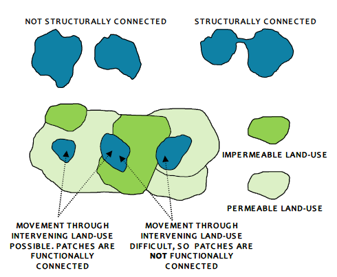
Figure 1. Contrast between structural and functional connectivity of habitat patches.
Click for a full description
Connectivity between habitat patches can be seen in both structural and functional contexts (Watts et al. 2005). Structural connectivity measures are based on the spatial distribution, size and number of fragments of habitat. In essence a structurally connected landscape is one where patches of habitat are directly linked so that species can move between patches of habitat without having to travel through the intervening habitat or matrix, which to a greater or lesser degree is unsuitable for the species in question.
Functional connectivity in contrast, does not require direct connections between patches or fragments, as long as the distances between patches are not so high, and intervening land-uses are not so hostile, as to prevent movement between patches. Intuitively, for some species, notably those with relatively poor dispersal abilities, certain types of land-use may be easier to move through than others, i.e. there are different ‘costs’ to an individual to movement through different land-uses. Land-use types may have a high cost to a particular species if they lack, for example, food or refuges, or have an increased risk of predation. Promotion of functional connectivity involves considering the extent to which it is possible to prioritise the conservation of existing relatively low-cost land-uses (i.e. those which are easy for a species to move through) between habitats, and promote changes in land-use through management interventions to reduce the cost of species movement.
4. Habitat network models
Habitat network modelling is a rapidly expanding area of research, and the following review can only introduce the main types of model which have been used. Readers requiring more detail are directed to the primary literature, for example Crooks & Sanjayan (2006); Saura & Pascual-Hortal (2007), Saura (2009).
Habitat network models share certain common characteristics. They all require a definition of what constitutes habitat for the species under consideration, both in terms of the type of habitat and the area required, and an estimate of the distances that can be travelled between patches. They differ in two main aspects. Some models simply consider the Euclidean distance between patches when calculating connectivity values, whereas other include information on how the intervening landscape modifies the potential for dispersal, which modifies the effective distance between the patches. Secondly, they differ substantially in how connections between patches are defined i.e. what measures are used to define connectivity.
4.1 Least-cost models
Least-cost models (e.g. Adriaensen et al. 2003; Humphrey et al. 2004; van Rooij et al. 2004; Moseley et al. 2008a,b; Latham & Gillespie 2009) are a specific type of graph-theory model, which are rooted in the notion of landscape permeability or resistance: the effect of land-use on ability of a species to move across the landscape. Different land-uses are assigned different permeability values, which reflect the relative cost or difficulty for a species to travel through that land-use.
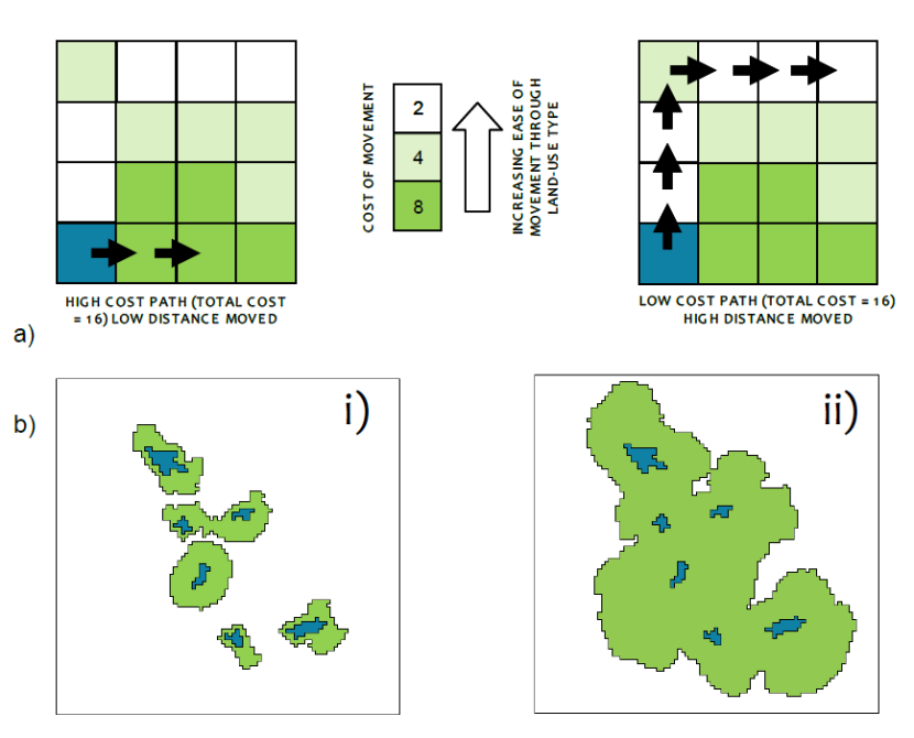
Figure 2. a) Illustration of the principle of least cost-modelling of habitat networks. This example shows two alternative paths through a landscape.
Click for a full description
They have the same total cost, but the distance travelled is very different due to the differing cost of the land-uses travelled through. b) Distances travelled away from habitat patches (blue) in i) a high cost landscape and ii) a low cost landscape.
Traversing an area of high-cost matrix will reduce the distance that a species is able to travel, and in extreme cases may prevent any movement i.e. be a complete barrier. This is known as the cost-distance and can be conveniently calculated in most GIS software applications using standard algorithms. The extent to which patches of habitat are connected depends on the nature of the intervening land-uses. Least-cost habitat networks are defined as those areas of land, including the habitat patches, where the cumulative cost of movement is less than the maximum distance that a species can travel. If the areas between two patches of habitat meet at any point then the patches are considered functionally connected (Moseley et al. 2008a).
4.2 Graph theory models
Two nodes are ‘linked’ if dispersal is possible between them, based on actual distance or cost distance. A large number of different indices have been developed to provide a quantification of the degree to which patches are connected (Saura and Pascal-Hortua 2007). These vary from simple measures such as the number of links between patches to more complex measures for example based on the number of links in the shortest paths between each connected patch relative to the number of nodes.
In addition to connectivity, graph theory models have been developed to evaluate the relative contribution of individual habitat patches to overall network connectivity (Saura & Rubio 2009).
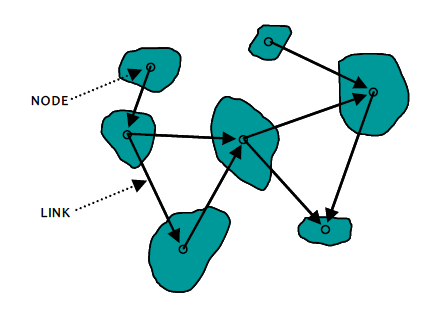
Figure 3. Illustration of a habitat network as envisaged through graph theory approaches. Nodes connected by links are part of the habitat network.
Click for a full description
Graph-theory models represent habitat networks as a series of nodes (patches) and edges (links) which make up the network graph (Urban & Keitt 2001; Pascual-Hortal & Saura, 2006; Figure 3).
4.3 Spatially-Explicit Population Models (SEPMs)
SEPMs (e.g. Macdonald & Rushton 2003; Graf et al. 2007; Suter et al. 2009) are based on a detailed understanding the population dynamics of species across a particular landscape. They can have varying degrees of complexity, but tend to model birth, death and dispersal processes explicitly based on patch areas and quality, inter-patch distances (actual or costdistances) and an assumed or measured dispersal probability curve, as opposed to least-cost or graph theory approaches which do not consider population dynamics.
SEPMs can be used to assess connectivity between patches by simulating the movement of individuals through the landscape based on the available understanding of the species movements. Although most closely representing reality, and therefore offering high predictive power when data are available, they are very difficult to parameterise, even for a single species and consequently have only limited application.
4.4 Habitat network models in the UK
At present in the UK, the majority of habitat network analyses that have been performed are based on least-cost models, principally generated by the BEETLE model developed by Forest Research (Watts et al. 2005; Moseley et al. 2008a,b). For this reason, the report will focus on the requirements of these models, but many of the areas explored subsequently are also relevant to other modelling frameworks due to the similarity of data utilised. A summary of the key information required to produce a least-cost habitat network is summarised below (Table 1).
| Information | Reason |
|---|---|
| Land use | Required to define habitat patches and assess effects of landscape on connectivity. |
| Species habitat preferences | Required to define the ‘source’ habitat patches, where the species can complete its life cycle. Can also incorporate patch area requirements. |
| Dispersal distance | Sets the maximum distance that can be traversed by species between habitat patches. |
| Permeability of land-uses | Required to determine the extent to which the intervening land-uses between habitat patches reduce the distance that can be travelled. ‘Habitat’ is assumed to have effectively no cost for dispersal. |
5. Extent of data supporting least-cost modelling of habitat networks
This section reviews the current extent of data which can be used to support the application of least-cost habitat network models, based on the requirements set out above.
Suitable data on land-uses are increasingly available in formats which are amenable for use in modelling (i.e. GIS layers), but there is substantial variation in the resolution, accuracy and completeness of the data available for different areas. Humphrey et al. (2005) review the range of datasets available for Scotland and the problems associated with their use. Different datasets may be most appropriate for analyses at different spatial scales, but naturally variation in the datasets used, such as the number of land-use categories distinguished and the extent to which categories can be related to priority habitats, can have a substantial effect on the outputs from network analyses.
Analyses can differ in the land-use types that are incorporated into distance calculations (Humphrey et al. 2005; Catchpole 2006; Moseley et al. 2008). This is particularly important in relation to low permeability, linear land-uses such as roads and railways, which may pose significant broad-front barriers to movement to many species (e.g. Rondinini & Doncaster 2002) but are not incorporated into all land-use datasets. Development of a consistent and up-to-date spatial land-use dataset is seen as a priority for future work (see section 9).
Despite the intuitive nature of the remaining requirements for undertaking a least-cost modelling analysis, obtaining suitable data on the species related parameters is not straightforward. Among the requirements, habitat preferences are probably the most well known. For many species these have been established either through existing autecological information or examination of distributional data in relation to land-use. There is a long history of gathering distributional data in the UK, and recent developments in access and delivery (e.g. the National Biodiversity Network) have aided the understanding of species habitat requirements. Broad habitat preferences established by these means may overestimate the extent of habitat and resultant networks, but at the same time more detailed information is often difficult to map onto the relatively broad land-use categories present in most spatial datasets.
Dispersal distances can be estimated through a number of different approaches, such as mark-release-recapture studies (Stasek et al. 2008), radio-tracking (Greenaway 2008), or indirect methods such as genetic relatedness of populations separated by differing distances or landscape features (Angelone & Holderegger 2008). There are inherent assumptions and uncertainties in all these methods (Clobert et al. 2001). Given the limited spatial and temporal extent of nearly all dispersal studies, particularly those involving direct measurement, they tend to measure the distances which most individuals move, yet fail to capture the rare, long-distance dispersal events, which may be of key importance in population persistence and colonisation. In addition, dispersal information tends to be most available for relatively common species, rather than those of conservation concern. A recent review of species in the UK found that only 28 out of 1245 species of conservation concern had published information on dispersal distances (Catchpole 2007).
Secondarily, but of key importance in least-cost models, is that dispersal distances are measured in a particular environment or landscape, which will have some influence on the distances measured. Given that dispersal is linked to the intrinsic permeability of the landscape it is measured in, estimates of these two parameters are often difficult to separate.
Assessment of the differential permeability of land-uses for a particular species, as required for least-cost models, would therefore ideally be based on empirical data on the movement of the species in question through the range of different environments which are present in the landscape under consideration. In a very few studies, this have been achieved (e.g. Driezen et al. 2007) but generally this kind of information is not available.
Eycott et al. (2008, 2010 in review) have recently reviewed the evidence base for the influence of matrix features (both different land-uses and particular features such as corridors or hedgerows) on dispersal. Considering the full extent of data that was available, meta-analysis indicated that there was evidence to support the intuitive view that dispersal between habitat patches was influenced by matrix features. This is consistent with other recent reviews for more specific taxonomic/habitat groups (e.g. Dover & Settele 2009 and Ochinger & Smith 2008 for butterflies; Browers & Newton 2009 for woodland invertebrates (mainly beetles)).
However, if the focus is brought more specifically to UK species, and considering situations where comparisons are available for distances moved between patches separated by different matrix types (at least two), the number of species for which data is available is very limited, and highly skewed taxonomically (see Table 2).
| Taxon | Mammals | Birds | Amphibians | Insects |
|---|---|---|---|---|
| Number of species | 1 | 29 | 1 | 4 |
Even where there is information available which may be relevant to habitat network modelling, it is sometimes highly variable or contradictory. Tables 3-6 below summarise relevant information for some relatively well studied UK species to which habitat network modelling is potentially relevant. For all species considered, for some parameters there is only a single estimate, and where there is more than one, there is considerable variation between estimates, leading to substantial uncertainty in parameter values.
| Information | Detail | Relevance for habitat network modelling | Source |
|---|---|---|---|
| Habitat preferences | Prefer highly diverse ancient deciduous woodland, but can also frequently be found in species-rich hedgerows and scrub. Can also occur in gardens and conifer plantations. Requires ancient woodland, but can disperse through all non-water habitats. | Some land-use data e.g. LCM2000 does not distinguish hedgerows, ancient deciduous woodland not always distinguished from other types, so habitat may be over-estimated. | Bright & Morris (1990) Bright et al. (2006) Macdonald & Rushton (2003) |
| Dispersal distances | Can travel at least 100m through non-habitat. Values of 0.1-2km suggested, 500m and 1.5km used in spatiallyexplicit population model. 250-500m across open ground between habitat patches. | Wide range of potential values for maximum dispersal distance – would have large influence on extent of network. | Bright (1998) Macdonald & Rushton (2003) Büchner (1997, 2008) |
| Permeability of land-uses | Faster movement through non-habitat (grass field), gaps in hedgerows can be barriers to movement. 55% crossed 1m gap, 6% 3m gap. | Not sufficient information to give reliable estimates of cost values for different land-uses. | Bright (1998) |
| Area requirement (home range) | 0.1-1km2 (home range) used in simulations. Populations found in woods of average area 2.9ha (± 1.4). | Wide range of potential values for minimum habitat area – would have large influence on number of suitable habitat patches | Macdonald & Rushton (2003) Büchner (2008) |
| Information | Detail | Relevance for habitat network modelling | Source |
|---|---|---|---|
| Habitat preferences | Marshy grassland, moorland and open woodland rides (marsh violets (Viola palustris) essential food plant). | Very specific habitat requirements; resolution of most land-use information not at this levels, so difficult to determine extent of suitable habitat. | Stewart & Bourn (2004), also Asher et al. (2001) |
| Dispersal distances | Mark-Release-Recapture, distances between 0.8-3.4km. | Maximum dispersal distance only from a study at a single site in a particular landscape configuration, so might not generalise. | Stewart & Bourn (2004) |
| Permeability of land-uses | Values used by Forest Research BEETLE model. | Sources of information used for derivation of cost-values unclear. | Kilpatrick (2005) |
| Area requirement | Occupied sites varied between 0.05 and 8.5ha. | Minimum area requirements only from a study at a single site in a particular landscape configuration, so might not generalise. | Stewart & Bourn (2004) |
| Information | Detail | Relevance for habitat network modelling | Source |
|---|---|---|---|
| Habitat preferences | Preference for different habitat types derived from kernel/Minimum Convex Polygon analysis of individual movements recorded by radio-tracking | Fine scale information, not easily translated to other more generally available land-use data | Greenaway (2008) McKenzie & Crowder (2009) |
| Dispersal distances | Direct measurement of distances moved from radio-tracking | Maximum dispersal distances derived from studies within similar landscape configurations, so might not generalise. | Greenaway (2008) McKenzie & Crowder (2009) |
| Information | Detail | Relevance for habitat network modelling | Source |
|---|---|---|---|
| Habitat preferences | Open coniferous forests, avoiding dense understory. Open areas within woodland required for lekking. Avoids areas close to tracks in woodland. | Density of coniferous forestry not generally distinguished in landuse classifications, so habitat may be overestimated. | Gjerde (1991) Sachot et al. (2003) Summers et al. (2007) |
| Dispersal distances | Dispersal to lekking sites, based on radio-tracking data. Males moved average of 2.3km, but some movements >7km. Dispersal distances generally between 5-10km. 1-30km natal dispersal by females in Deeside (median 11km). | Wide range of potential values for maximum dispersal distance – would have large influence on extent of network. | Hjeljord et al. (2000) Storch & Segelbacher (2000) Moss et al. (2000) |
| Permeability of land-uses | Mountain ranges act as barriers, land-use does not influence dispersal, based on landscape genetic study. | Most land-uses have low cost, but elevation needs to be incorporated as a modifier of cost to movement. | Kormann (2009) |
| Area requirement | Adult males mean home range 63.5ha, females 26.8ha. | Derived from a single study, so may not generalise, sex differences may affect estimation of the extent of habitat. | Gjerde & Wegge (1989) |
6. Uncertainty in least-cost habitat networks: how best to proceed
Due to the current limitations of data available to support modelling, a situation which is unlikely to change substantially in the short to medium term, it is essential that appropriate strategies are employed to minimise and account for the effects of uncertainty in habitat network analyses.
6.1 Uncertainty in parameters
There is uncertainty in all parameters involved in modelling, but probably the most uncertainty is linked to estimates of landscape permeability. Two recent studies have examined the effect of uncertainty in permeability values on least-cost habitat network configuration (Beier et al. 2009; Rayfield et al. 2009). The study by Beier et al (2009) focused on networks for large mammal species in southern California, whereas the Rayfield et al. (2009) study was based on simulated landscapes of differing fragmentation.
In both studies changes in the permeability or resistance values caused in
some cases considerable shifts in the extent to which patches were connected and the spatial location of identified areas of functional connectivity. The study by Beier et al. (2009) found that for five out of eight species considered the assessment of connectivity was robust, but for the other three species the overlap between networks identified using different, but plausible, combinations of permeability values was as little as 0%, although the mean overlap was 78%. These differences could not be easily attributed to biological or ecological differences between the taxa under consideration. Rayfield et al. (2009), through using simulated landscapes, found that sensitivity of network configuration was greatest in highly fragmented landscapes, precisely where networks are potentially of greatest importance in promoting persistence.
Both studies found that it was the relative (i.e. rank-order), rather than the absolute permeability values which were important in determining the configuration of resultant networks. This would suggests that as long as relative permeability values are broadly appropriate, the relative extent of different networks should be reasonable robust, although it is not appropriate to place too much weight on this conclusion given that it is based on only two studies. For on-the-ground planning, it is important to emphasise that actual functional connectivity between patches will only be accurate where all the parameters involved are valid.
6.2 Expert opinion and the Delphi process
Owing to the lack of empirical data, expert opinion is widely used to derive estimates of parameters such as dispersal distances and landscape permeability. However, estimates derived from different experts can commonly vary widely (Catchpole 2007, Watts et al. 2008, see also Table 8) and expert opinion should be incorporated through a Delphi process wherever possible.
A Delphi process is a procedure used to gather data from experts and build a consensus on a given issue (Macmillan & Marshall 2006). The initial step is to ask a panel of experts to independently give an assessment of an issue (in the case of habitat networks, an estimate of dispersal distance or permeability of different land-uses) and the reasoning for their assessment. The responses are collated and summarised by a facilitator and a summary is sent to all members of the expert panel. They are then asked to consider their responses in the light of the responses and reasoning put forward by all the other participants and submit a revised response and reasoning. This process is repeated up to a further two times to allow for iterative changes of position. The final result of the process is consensus or a reduced range of responses, with reasoning behind any deviation from consensus.
The Delphi process has been used in a wide range of fields such as IT project risk assessment (Skulmoski et al. 2007), nursing and health care practice (Akins et al. 2005) and policy making (Rayens & Hahn 2000), in addition to estimation of parameters for ecological modelling (MacMillan & Marshall 2006; Watts et al. 2008). Whilst it has been widely used, there has been little or no assessment of the accuracy of the estimates obtained in the light of increased availability of data on the process under consideration.
The general objective of a Delphi process is consensus, but for habitat network modelling, given the underlying uncertainty in many of the parameters for which a Delphi process may be used to derive estimates, the range of values that are provided may be more appropriate for use in network analysis, producing maximum and minimum estimates of network extent and configuration and allowing the effects of uncertainty to be examined. This is similar to the ‘worst-case’ scenario used by Beier et al. (2009) in their assessment of habitat network stability in relation to changes in parameters.
Ironically for a method which seeks to build consensus, there is no consensus in the literature on an appropriate number of participants in the process. Examples in the literature range from 3 to over 1000 (Akins et al. 2005; Hsu & Sandford, 2007; Skulmoski et al. 2007). A minimum of 10 participants has been suggested, but there is no strong basis for this number. Clearly as in most situations, a larger sample size improves the potential for capturing the range of opinion and expertise, and thus for variation in estimates, and reduces the likelihood of bias through selection of participants who share similar viewpoints. When the participants are from heterogeneous backgrounds it may be advantageous to increase the sample size if possible (Skulmoski et al. 2007). In many cases relevant to habitat network models, the number of people sufficiently expert in taxa under consideration is likely to be severely limited. In addition, the criteria that can be used for participant selection are ambiguous (Hsu & Sandford 2007), which further limits the scope for objective recommendations.
For more detail on the Delphi process, the standard text is Linstone & Turoff (1975), which provides encyclopaedic coverage of the subject.
6.3 The use of Generic Focal Species
Required data for any particular species is very limited in almost all cases. This, along with the fact that in most cases conservation efforts are required to have benefits for more than one species, has lead to the widespread use of Generic Focal Species (GFS) (Eycott et al. 2007) for modelling purposes. GFS are ‘designed’ to represent a range of species of conservation interest within the particular landscape or habitat e.g. woodland generalists with moderate dispersal ability, or heathland specialists with low dispersal ability (see Table 7). GFS are given dispersal distances and land-use permeability values which are intended to capture general patterns rather than specific actual species, again derived from expert opinion.
| Species | Habitat preferences | Dispersal distance | Indicative landscape permeability |
|---|---|---|---|
Broad-leaved woodland specialist | Broad-leaved woodland | 1km | Other woodland types permeable, but other land-uses generally low permeability |
| Grassland generalist | Natural grassland of any kind | 0.5-2km | Urban areas and water low permeability, plantation forestry and improved pasture medium, open woodland and improved grassland highly permeable |
The use of GFS is inevitable when faced with the paucity of empirical data, but it is important to appreciate that even when a GFS profile is closely aligned to the set of species under consideration, the resultant habitat network is unlikely to perform equally well for all species in terms of actual connectivity between patches of habitat. Habitat network modelling is not suited to all types of species, with the emphasis being largely placed on those species with traits that make them vulnerable to fragmentation effects (Watts et al. 2005). Species with other combinations of traits, such as highly mobile, or highly sedentary, species, may show less dependence on ‘network’ processes for persistence. Conservation of these species will require the consideration of alternative strategies. It is therefore important in initial planning and setting of objectives to ensure that habitat network modelling is an appropriate tool to employ.
7. Representing uncertainty in the outputs of least-cost network analyses
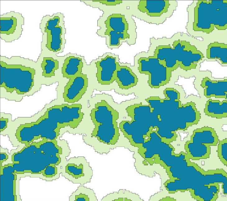
Figure 4. Example of nested habitat networks generated by setting maximum dispersal distance to 500m (blue), 1km (dark green) and 2km (pale green) respectively.
Click for a full description
It is vital that the outputs of least-cost habitat network analyses are communicated and interpreted in a way which effectively represents the underlying uncertainty in analyses. Uncertainty has been incorporated in previous analyses largely through varying the maximum dispersal distance of the GFS (e.g. Moseley et al. 2008a), which generates a series of nested networks, representing the change in network configuration that occurs with differing maximum dispersal distance.
The national analysis of Forest Habitat Networks (FHN) in Scotland (Moseley et al 2008b) undertook a sensitivity analysis of the outputs from the BEETLE least-cost model, based on a 20% change (both increase and decrease) in permeability values. The sensitivity analysis considered the influence of this variation in permeability on the number of networks (i.e. the number of sets of habitat patches that were considered to be functionally connected) and total network area (all networks combined), finding that there was generally fairly low variability in the results. However there was no assessment of changes in location of networks, which has more important consequences for land-use planning and prioritisation of conservation interventions. Secondly, as all permeability values were modified in the same direction (increase or decrease) and by the same amount, their rank order was not altered and hence only a minor change would be expected (Beier et al., 2009; Rayfield et al., 2009). Changes to one or more high-cost land-use permeability values, rather than varying them all together, may have a bigger impact on the results of the network analysis.
In existing applications of least-cost models in the UK (e.g. Catchpole 2006, 2007, Moseley et al. 2008a,b), the limitations of least-cost analyses are clearly and repeatedly acknowledged and highlighted, with emphasis placed on the ‘fuzziness’ inherent in the resultant network maps and the importance of considering this when interpreting the network analyses for land-use planning. However the impact of this uncertainty is not well communicated when simply viewing the network maps, which in general place clear and well defined boundaries on the habitat networks, and only give outputs based on either single estimates or mean/median permeability values, with no visual indication of the underlying uncertainty. In addition, parameter uncertainty will not affect all parts of the network configuration equally and it would be highly valuable to be able to assess which parts of a habitat network are more or less robust to variation in parameters.
A simple but effective way to explore the implications of uncertainty in parameters is to derive least-cost networks utilizing a range of values for permeability and dispersal distances. It is possible to generate maps that illustrate the maximum and minimum networks (i.e. maximum dispersal distance and permeability values and minimum dispersal distance and permeability values) to illustrate the effects of uncertainty on network configuration and also areas which are particularly affected by the uncertainty This is akin to the ‘worst-case scenario’ analysis undertaken by Beier et al. (2009). The example shown in Figure 4 shows maximum and minimum networks for a broad-leaved specialist species based on the range of permeability values derived from a Delphi analysis (Table 8: Watts et al. 2008) and a dispersal range of 1-2km.
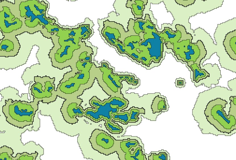
Figure 5. Habitat networks for a broad-leaved woodland specialist species, based on maximum (pale green), mean (mid green) and minimum (dark green) permeability values derived from a Delphi analysis, see Table 8,
Click for a full description
and maximum dispersal distances of 500m, 1km and 2km respectively. Blue indicates habitat patches. Differences in total area of habitat networks shown: maximum permeability, 2km dispersal = 2141ha, mean permeability, 1km dispersal = 1220ha, minimum permeability, 500m dispersal = 655ha.
As can be clearly seen, there is considerable variation in the extent to which individual fragments of broad-leafed woodland are functionally connected depending on the combination of permeability and dispersal parameters used. Some parts of the network exhibit greater variability than others. This emphasises that effects of changes in dispersal distances or permeability values are strongly context dependent, even within a single habitat network application.
| Broad Habitat class | Min | Max | Mean |
|---|---|---|---|
| Acid grassland | 12 | 30 | 25 |
| Arable and horticulture | 33 | 50 | 47 |
| Bog | 14 | 50 | 29 |
| Boundaries and linear features | 14 | 20 | 16 |
| Broad-leaved, mixed and yew woodland | 1 | 1 | 1 |
| Bracken | 12 | 29 | 18 |
| Built-up areas and gardens | 14 | 50 | 33 |
| Calcareous grassland | 26 | 50 | 33 |
| Coniferous woodland | 7 | 29 | 18 |
| Dwarf shrub heath | 12 | 29 | 19 |
| Fen, marsh and swamp | 12 | 29 | 19 |
| Improved grassland | 33 | 50 | 47 |
| Inland rock | 5 | 50 | 24 |
| Littoral rock | 50 | 50 | 50 |
| Littoral sediment | 50 | 50 | 50 |
| Montane habitats | 26 | 50 | 35 |
| Neutral grassland | 26 | 50 | 33 |
| Rivers, streams | 14 | 50 | 34 |
| Road linear features | 14 | 50 | 35 |
| Standing open water and canals | 12 | 50 | 32 |
| Supra-littoral rock | 50 | 50 | 50 |
| Supra-littoral sediment | 50 | 50 | 50 |
8. Appropriate use of least-cost habitat network models
With the increasing pressure on natural and semi-natural landscapes throughout the world, it will not be feasible to wait until suitable data are available for all species of conservation interest to undertake habitat network analyses and guide decision making. In order to be able to make pragmatic and informed decisions about when and how to use habitat network models, consideration should be given to the situations where habitat networks are an appropriate technique and also the limitations described previously.
Habitat network models are one potentially powerful tool for contributing to the conservation of biodiversity through effective landscape management, but as is the case for any conservation technique, they should not be used without due consideration or in isolation from other criteria and considerations. To this end Table 9 provides a summary of issues that should be considered before using habitat network models, and Table 10 gives some examples of the type of questions that could be addressed using habitat network models and an indication of the confidence that should be associated with the outputs in different applications, based on the current evidence base.
| Question to be asked | Implications |
|---|---|
| Are the species under consideration likely to benefit from a habitat network approach? | Not all species are likely to benefit from habitat networks. As Watts et al. (2005) indicate, relevant considerations are the dispersal ability and habitat area requirements of the species. Habitat networks are likely to have the greatest benefit for species with moderate dispersal abilities and relatively high area requirements, as these are the species that are sensitive to habitat fragmentation. Species with very poor or very good dispersal abilities are unlikely to benefit significantly from habitat network approaches. It is difficult to generalise across taxonomic groups, but there is evidence that is consistent with the use of habitat networks for woodland invertebrates (e.g. Bailey 2007), butterflies (e.g. Thomas & Hanski 1993) and amphibians (e.g. Joly et al. 2000). |
| Is there sufficient information available? | As indicated previously, the data sources that are used to derive habitat networks, regardless of the technique used, have a substantial effect on the outputs. |
| What are the alternatives to least-cost habitat networks? | As Hodgson et al. (2009, 2011) point out, effective management of habitats for conservation involves consideration of habitat area, quality and connectivity as appropriate. Habitat networks aim to improve connectivity, but this is only one potential strategy, and the evidence base for positive effects of increasing connectivity is relatively small compared to that demonstrating positive effects of increasing habitat area or quality. These alternatives should therefore always be considered as well as networks when examining conservation strategies. |
| What is the question to be addressed? | General confidence in outputs | What should you particularly consider? |
|---|---|---|
What is the current habitat network for a particular species?
| Low | Do the biological traits of the species under consideration make it likely to benefit from habitat networks? Data required is very limited for most species. Consider undertaking detailed research on focal species to establish appropriate parameters. |
Which habitats have the most extensive intact networks?
| Medium | Use a range of GFS profiles to capture uncertainty in values. Broad-scale analyses are likely to be most robust. |
Where should I prioritise land management to improve networks? | Medium | Boundaries of networks are intrinsically ‘fuzzy’ and land management outside the network boundaries will not necessarily produce lesser returns. Use a range of values in network analyses to assess uncertainty of locations. |
| Where is there overlap between habitat networks for different species? | Medium | Areas of overlap will depend on parameters used so use a range of profiles Overlapping parts of networks are unlikely to form suitable habitat for different species considered, so conservation of these areas may not give best return |
| What is the effect of alternative land-use changes on habitat networks? | High | Outputs can be used as one criterion for ranking and assessment of alternatives GFS profiles should be closely aligned to species considered for maximum benefit |
9. Future priorities for research and development
Habitat network modelling is a rapidly developing area of science, but as in many other cases, the development of models has far outstripped the availability of data. This situation is unlikely to change substantially in the foreseeable future, but there are a number of areas where focusing research may have benefits in guiding more effective use of habitat network models.
9.1 Landscape genetics
This is an area of research which may provide alternative way of providing estimates of parameters for habitat network models. An extension of population genetics, it attempts to link the genetic relatedness of populations to the landscape matrix that separates them, rather than base calculations on purely isolation by distance.
The increasing availability of analytical tools and genetic primers for a range of species makes this a potentially valuable area for improving our understanding of how landscape composition affects the movement of individuals in different situation. There have already been some successful applications of landscape genetics to modelling analyses (e.g. Angelone & Holderegger 2008; Kormann 2009).
Thee are however important questions that remain to be answered regarding the use of landscape genetics. Of particular relevance is the extent to which patterns of genetic relatedness reflect contemporary landscape configurations rather than past patterns (e.g. Orsini et al. 2008). Given the speed of landscape change in many areas of the world, it is unlikely that population genetics are in equilibrium with the current landscape, complicating interpretation of observed patterns.
9.2 Use of distributional data to determine landscape permeability
The UK has a large and rapidly increasing archive of distributional information for a wide range of taxa (e.g. the National Biodiversity Network). This information is potentially highly valuable for habitat network modelling, but is currently not being exploited to its full potential. Janin et al. (2009) have recently developed a method that can calibrate permeability values of a landscape based on distributional data. One potential problem with this approach is that it assumes that distribution reflects ability to disperse through a particular land-use (Horskins et al. 2006). This may not be valid for species that are highly dispersive, but for less highly mobile species such many invertebrates and plants which may have to survive in intervening habitats rather than simply dispersing rapidly through them, this may prove to be a valid approach and worthy of further research.
9.3 Developing consistent spatial land-use databases:
The current variety of spatial land-use information makes it difficult to compare results of different analyses. Throughout the UK, Phase 1 habitat information (JNCC 2010) is being gathered and collated by local authorities and other bodies. This would potentially provide a consistent and relatively high spatial resolution dataset which could form the basis of habitat network analyses. However at present, the completeness and availability of the data is variable, with some areas only having paper-based resources and efforts to develop a consistent national scale dataset would have benefits for habitat network modelling amongst other applications.
9.4 Integration of alternative modelling frameworks
As indicated in previous sections, there are a wide and ever increasing range of potential habitat network models for a potential user to select from (see McRae et al. 2008 for a recent development). Most of the existing analyses in the UK have used least-cost models, at least partly due to their ease of access in most GIS environments, rather than necessarily because they are the most appropriate model for the application. As the number of models increases, it is important to attempt to evaluate whether different modelling frameworks are particularly applicable to certain situations or species, based on their dispersal mode, behaviour or other attributes. There has been little attempt to date to perform comparative analyses of different models, to highlight areas where they are most similar or divergent in their predictions and to use this to guide appropriate application of the different models.
10. Technical details of habitat network models used
All habitat network maps were created using standard cost-distance algorithms implemented in a GIS environment (ITC-ILWIS, 2001). Land-use data was derived from Land Cover Map 2000 data for Scotland, used under SNH license from the Centre for Ecology and Hydrology, in combination with road data from the Ordnance Survey Meridian 2 dataset (© Crown Copyright and database right 2011).
11. Acknowledgements
The following individuals are acknowledged for contributing data, information, manuscripts or advice during the current project: Kevin Watts and Amy Eycott (Forest Research), Nigel Bourn (Butterfly Conservation), Ron Summers (RSPB), Rich Howorth (West Weald Landscape Project) and Sven Büchner.
12. References
Akins, R.B., Tolson, H. & Cole, B.R. (2005) Stability of response characteristics of a Delphi panel: application of bootstrap data expansion. BMC Medical Research Methodology 5, 37.
Angelone, S. & Holderegger, R. (2008) Population genetics suggests effectiveness of habitat connectivity measures for the European tree frog in Switzerland. Journal of Applied Ecology 46, 879-887.
Araujo, M.B., Cabeza, M., Thuiller, W., Hannah, L. & Williams, P.H. (2004) Would climate change drive species out of reserves? An assessment of existing reserve-selection methods. Global Change Biology 10, 16181626.
Asher, J., Warren, M., Fox, R., Harding, P., Jeffcoate, G., Jeffcoate, S. (2001) The millennium atlas of butterflies in Britain and Ireland. Oxford University Press, Oxford.
Bailey, S. (2007) Increasing connectivity in fragmented landscapes: an investigation of evidence for biodiversity gain in woodlands. Forest Ecology and Management 238, 7-23.
Beier, P., Majka, D.R. & Newell, S.I. (2009) Uncertainty analysis of least-cost modelling for designing wildlife linkages. Ecological Applications 19, 2067–2077.
BRANCH partnership (2007) Planning for biodiversity in a changing climate – BRANCH project Final Report, Natural England, UK.
Bright, P. W. & Morris, P. A. (1990) Habitat requirements of dormice Muscardinus avellanarius in relation to woodland management in Southwest England. Biological Conservation 54, 307-326.
Bright, P. W., Morris, P. A. & Mitchell-Jones, A. J. (2006) The Dormouse
Conservation Handbook, second edition. Peterborough: English Nature.
Bright, P.W. (1998) Behaviour of specialist species in habitat corridors:
arboreal dormice avoid corridor gaps. Animal Behaviour 56, 1485-1490.
Brouwers, N.C.& Newton, A.C. (2009) Movement rates of woodland invertebrates: a systematic review of empirical evidence. Insect Conservation and Diversity 2, 10–22.
Büchner, S. (1997) Common dormice in small isolated woods. Natura Croatica 6, 271-274.
Büchner, S. (2008) Dispersal of common dormice Muscardinus avellanarius in a habitat mosaic. Acta Theriologica 53, 259-262.
Catchpole, R.D.J. (2006) Planning for biodiversity - opportunity mapping and habitat networks in practice: a technical guide. English Nature Research Report 687, English Nature, Peterborough.
Catchpole, R.D.J. (2007) England Habitat Network Information Note. Natural England Internal Briefing Note.
Clobert, J., Danchin, E., Dhondt, A.A. & Nichols, J.D. (2001) Dispersal.
Oxford University Press, Oxford.
Crooks, K.R. & Sanjayan, M. (eds.) (2006) Connectivity Conservation. Cambridge University Press, Cambridge.
Diamond, J.M. (1975) The island dilemma: lessons of modern biogeographic studies for the design of nature reserves. Biological Conservation 7,129–145.
Doerr, V.A.J., Barrett, T. & Doerr, E.D. (2011) Connectivity, dispersal behaviour and conservation under climate change: a response to Hodgson et al. Journal of Applied Ecology 48, 143-147.
Donald, P.F., Sanderson, F.J., Burfield, I.J., Bierman, S.M., Gregory, R.D. & Waliczky, Z. (2007) International conservation policy delivers benefits to birds in Europe. Science 317, 810-813.
Dover, J. & Settele, J. (2009) The influences of landscape structure on butterfly distribution and movement: a review. Journal of Insect Conservation 13, 3-27.
Driezen, K., Adriaensen, F., Rondinini, C., Doncaster, C.P., & Matthysen, E. (2007) Evaluating least-cost model predictions with empirical dispersal data: A case-study using radiotracking data of hedgehogs (Erinaceus europaeus). Ecological Modelling 209, 314-322.
Eycott, A.E., Watts, K., Moseley, D.G. and Ray, D. (2007). Evaluating Biodiversity in Fragmented Landscapes: The Use of Focal Species. Forestry Commission Information Note No.089, Forestry Commission, Edinburgh.
Eycott, A., Watts, K., Buyung-Ali, G., Bowler, D., Stewart, G. & Pullin, A (2008) Which landscape features affect species movement? A systematic review in the context of climate change. Final Report of DEFRA Research contract CR0389.
Eycott, A., Watts, K., Buyung-Ali, G., Bowler, D., Stewart, G. & Pullin, A (2010, in review) Which matrix features affect species movement? Collaboration for Environmental Evidence, Systematic Review No. 43 Draft Review Report.
Gjerde, I. & Wegge, P. (1989) Spacing pattern, habitat use and survival of Capercaillie in a fragmented winter habitat. Ornis Scandinavica 20, 219225.
Gjerde, I. (1991) Cues in winter habitat selection by Capercaillie. I. Habitat characteristics. Ornis Scandinavica 22, 197-204.
Graf, R.F., Kramer-Schadt, S. Fernandez, N. & Grimm, V. (2007) What you see is where you go? Modeling dispersal in mountainous landscapes. Landscape Ecology 22, 853-866.
Greenaway, F. (2008) Barbastelle bats in the Sussex West Weald 1997 - 2008. Report to Sussex Wildlife Trust.
Hanski, I. & Gilpin, M.E. (eds.) (1997) Metapopulation Biology: Ecology, Genetics & Evolution. Academic Press, London.
Hanski I., Pakkala, T, Kuussaari, M, & Lei G. (1995). Metapopulation persistence of an endangered butterfly in a fragmented landscape.
Oikos, 72, 21-28.
Hjeljord, O., Wegge, P., Rolstad, J., Ivanova, M. & Beshkarev, A.B. (2000) Spring-summer movements of male capercaillie Tetrao urogallus: A test of the 'landscape mosaic' hypothesis. Wildlife Biology 6, 251-256.
Hodgson, J.A., Thomas, C.D., Wintle, B.A. & Moilanen, A. (2009) Climate change, connectivity and conservation decision making: back to basics. Journal of Applied Ecology 46, 964-969.
Hodgson, J.A., Moilanen, A., Wintle, B.A. & Thomas, C.D. (2011) Habitat area, quality and connectivity: striking the balance for efficient conservation. Journal of Applied Ecology 48, 148-152.
Horskins, K., Mather, P.B. & Wilson, J.C. (2006) Corridors and connectivity: when use and function do not equate. Landscape Ecology 21, 641-655.
Humphrey, J., Ray, D., Watts, K., Brown, C., Poulsom, L., Griffiths, M. & Broome, A. (2004). Balancing upland and woodland strategic priorities.
Scottish Natural Heritage Commissioned Report No. 037 (ROAME No. F02AA101).
Humphrey, J., Watts, K., McCracken, D., Shepherd, N., Sing, L., Poulsom, L., Ray, D. (2005). A review of approaches to developing Lowland
Habitat Networks in Scotland. Scottish Natural Heritage Commissioned
Report No. 104 (ROAME No. F02AA102/2)
Hsu, C.C. & Sandford, B.A. (2007) The Delphi technique: making sense of consensus. Practical Assessment, Research and Evaluation 12, 10.
ITC-ILWIS (2001) ILWIS 3.0 User’s Guide: Chapter 9. Spatial data analysis:
neighbourhood and connectivity calculations. ITC-ILWIS, The Netherlands.
JNCC (2010) Handbook for Phase 1 habitat survey – a technique for environmental audit. Joint Nature Conservation Committee, Peterborough.
Kharouba, H.M. & Kerr, J.T. (2010) Just passing through: Global change and the conservation of biodiversity in protected areas. Biological Conservation 143, 1094-1101.
Kirkpatrick, A. (2005) Assessment of the metapopulation dynamics of the small pearl-bordered fritillary (Boloria selene) in Clocanenog and Alwen forests, North Wales. MSc Dissertation, University of Wales.
Koormann, U.G. (2009) Landscape genetics in capercaillie (Tetrao urogallus L.): Combining direct and indirect methods to quantify dispersal and functional connectivity in a mountain landscape. MSc Dissertation, University of Bern.
Latham, J. & Gillespie J (2009) Applying connectivity mapping to spatial planning in Wales. In: Catchpole, R (ed.) Ecological Networks: Science and Practice. Proceedings of the Sixteenth Annual IALE (UK) Conference, Edinburgh University, Edinburgh.
Linstone, H. A., & Turoff, M. (eds.). (1975) The Delphi method: Techniques and application. Reading, MA: Addison-Wesley.
MacArthur R.H. & Wilson E.O. (1967) The Theory of Island Biogeography.
Princeton University Press, Princeton.
Macdonald, D.W. & Rushton, S (2003) Modelling space use and dispersal of mammals in real landscapes: a tool for conservation. Journal of Biogeography 30, 607-620.
MacMillan, D.C. & Marshall, K. (2006) The Delphi process – an expert-based approach to ecological modelling in data-poor environments. Animal Conservation 9, 11-19.
McKenzie, S. & Crowder, K. (2009) Developing a land management targeting framework for the West Weald Project area. Report prepared for Sussex Wildlife Trust.
McRae, B.H., Dickson, B.G., Keitt, T.H. & Shah, V.B. (2008) Using circuit theory to model connectivity in ecology and conservation. Ecology 89, 2712-2724.
Millennium Ecosystem Assessment, 2005. Ecosystems and Human Wellbeing: Biodiversity Synthesis. World Resources Institute, Washington, DC.
Moilanen, A., Smith, A.T. & Hanski, I. (1998) Long-term dynamics in a metapopulation of the American Pika. American Naturalist 152, 530-542.
Moseley, D., Ray, D., Watts, K. & Humphrey, J. (2008a) Forest Habitat Networks Scotland: Final Report. Contract report to Forestry Commission Scotland, Forestry Commission GB and Scottish Natural Heritage.
Moseley, D., Smith, M., Chetcuti, J. & de Ioanni, M. (2008b) Falkirk Integrated Habitat Networks. Contract report to Falkirk Council, Forestry Commission Scotland, Scottish Natural Heritage, and Central Scotland Forest Trust.
Moss, R., Picozzi, N. & Catt, D. C. (2006) Natal dispersal of capercaillie Tetrao urogallus in northeast Scotland. Wildlife Biology 12, 227-232.
Ockinger, E. & Smith, H. G. (2008) Do corridors promote dispersal in grassland butterflies and other insects? Landscape Ecology 23, 27-40.
Orsini, L., Corander, J., Alasentie, A. & Hanski I. (2008) Genetic spatial structure in a butterfly metapopulation correlates better with past than present demographic structure. Molecular Ecology 17, 2629-2642.
Pascual-Hortal, L. & Saura, S. (2006) Comparison and development of new graph based landscape connectivity indices: towards the priorization of habitat patches and corridors for conservation. Landscape Ecology 21, 959–967.
Pope, S.E., Fahrig, L. & Merriam, H.G. (2000) Landscape complementation and metapopulation effects on leopard frog populations. Ecology 81, 2498-2508.
Prugh, L.R., Hodges, K.B., Sinclair, A.R.C & Brashares, J.S. (2009) Effect of habitat area and isolation on fragmented animal populations. Proceedings of the National Academy of Sciences of the USA 105, 20770-20775.
Rayens, M.K. & Hahn, E.J. (2000) Building consensus using the Delphi policy method. Policy, Politics and Nursing Practice 1, 308-315.
Rayfield, B., Fortin, M-J. & Fall, A (2009) The sensitivity of least-cost habitat graphs to relative cost surface values. Landscape Ecology 25, 519-532.
Rodrigues, A.S.L., Andelman, S.J., Bakarr, M.I., Boitani, L., Brooks, T.M., Cowling, R.M., Fishpool, L.D.C., da Fonseca, G.A.B., Gaston, K.J.,
Hoffmann, M., Long, J.S., Marquet, P.A., Pilgrim, J.D., Pressey, R.L.,
Schipper, J., Sechrest, W., Stuart, S.N., Underhill, L.G., Waller, R.W., Watts, M.E.J. & Yan, X. (2004) Effectiveness of the global protected area network in representing species diversity. Nature 428, 640-643.
Rondinini, C. & Doncaster, C.P. (2002) Roads as barriers to movement of hedgehogs. Functional Ecology 16, 504-509.
Sachot, S., Perrin, N. & Neet, C. (2003) Winter habitat selection by two sympatric forest grouse in western Switzerland: implications for conservation. Biological Conservation 112, 373-382.
Saura, S. (2009) Measuring connectivity in landscape networks: towards meaningful metrics and operational decision support tools. In: Catchpole, R., Smithers, R., Baarda, P. & Eycott, A. (eds.) (2009) Ecological Networks: Science and Practice, 1-10.
Saura, S. & Pascual-Hortal, L. (2007) A new habitat availability index to integrate connectivity in landscape conservation planning: comparison with existing indices and application to a case study. Landscape and Urban Planning 83, 91-103.
Saura, S. & Rubio, L. (2010) A common currency for the different ways in which patches and links can contribute to habitat availability and connectivity in the landscape. Ecography (in press).
Skulmoski, G.J., Hartman, F.T. & Krahn, J. (2007) The Delphi method for graduate research. Journal of Information Technology Education 6
Soulé, M. (ed.) (1987) Viable populations for conservation. Cambridge University Press, Cambridge.
Summers, R.W., McFarlane, J. & Pearce-Higgins, J.W. (2007) Measuring avoidance by capercaillies Tetrao urogallus of woodland close to tracks. Wildlife Biology 13, 19-27.
Suter, W., Bollmann, K. & Holderegger, R. (2009) Landscape permeability: from individual dispersal to population persistence. In: Kienast, F., Wildi, O. & Ghosh, S. (eds.) A Changing World. Challenges for Landscape Research, 157–174.
Stasek, D.J., Bean, C. & Crist, T.O. (2008) Butterfly abundance and movements among prairie patches: the roles of habitat quality, edge, and forest matrix permeability. Environmental Entomology 37, 897-906
Stewart, K.E.J. & Bourn, N.A.D. (2004) The status, mobility and habitat requirements of the small pearl-bordered fritillary (Boloria selene) in
Clocaenog Forest: an overview of three years work. Butterfly
Conservation Contract Report to Forest Research Report No. SO4-11.
Storch, I. & Segelbacher, G. (2000) Genetic correlates of spatial population structure in central European capercaillie Tetrao urogallus and black grouse T. tetrix: a project in progress. Wildlife Biology 6, 305-310.
Taylor, P.D., Fahrig, L., Henein, K. & Merriam, G. (1993). Connectivity as a vital element of landscape structure. Oikos 68, 571-573.
The Wildlife Trusts (2006) Living Landscapes: a call to restore the UK's battered ecosystems for wildlife and people. The Wildlife Trusts, Newark, Nottinghamshire.
Urban, D. & Keitt, T.H. (2001) Landscape connectivity: a graph theoretic perspective. Ecology 82, 1205–1218.
van Rooij S, van der Sluis T, Steingrover E, Clarke S (2004) Applying landscape ecological methods to analyse and design ecological networks. In: Smithers, R. (ed) Landscape Ecology of Trees and Forests. Proceedings of the Twelth Annual IALE (UK) Conference, Royal Agricultural College, Cirencester, England.
Vos, C.C., Verboom, J., Opdam, P. F. M. & Ter Braak, C. J. F. (2001) Toward ecologically scaled landscape indices. American Naturalist, 183, 24-41.
Watts, K., Humphrey, J., Griffiths, M., Quine, C., and Ray, D. (2005).
Evaluating Biodiversity in Fragmented Landscapes: Principles. Information Note 73, Forestry Commission, Edinburgh.
Watts, K., Handley, P., Scholefield, P. & Norton, L. (2008) Habitat Connectivity – Developing an indicator for UK and country level reporting. Phase 1 Pilot Study. Final report for DEFRA Research Contract CR0388.