Big Biodiversity Layer Development

The Big Biodiversity Layer (BBL) is a tool which is being developed at NatureScot to map biodiversity across Scotland, in order to identify the most highly biodiverse areas which need protection. The BBL is intended to be one tool which helps inform decision making around new 30x30 sites. We are developing this tool with a focus on identifying Other Effective area-based Conservation Measures (OECMs), and are using the criteria for these as guidance. The finished product will identify areas which should be explored to confirm a high level of biodiversity, and it will benefit the bottom-up approach as it will allow landowners to assess their own land for areas with OECM potential. 

Proposed Big Biodiversity Layer methodology

The BBL will initially focus on each “important for biodiversity” value separately and produce a heat map for each of these. To do this, combinations of species and habitats (selected for their relevance to each criteria), will be weighted against the different values and mapped with points/polygon data. For example, species and habitats which can be considered rare, threatened or endangered will fit the first criteria and can be weighted according to red lists and nationally scarce/nationally rare lists. Combinations of different datasets will be used, largely looking at data from NBN Atlas for species, and datasets like HabMoS for mapped habitats. 

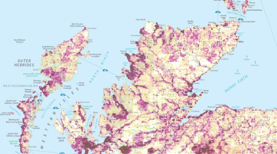
Scotland will be split into a 1km x 1km grid; with each square summing up weightings from any species or habitats present within it and producing a “biodiversity value”. 

We are working iteratively, layers produced sequentially and combined as they become available. We intend to use a hot spot analysis to identify areas with the highest biodiversity values, taking a higher-level approach to focus on areas with neighbouring grid squares of consistently high value. This means that to be a statistically significant hotspot, features of high values will be surrounded by other features of high value. It will target high value areas of biodiversity at a larger (landscape?) scale. 

With the complete set of layers combined, we will have a layer broadly summarising the levels of biodiversity across Scotland – the Big Biodiversity Layer! 

Big Biodiversity Layer use

With the completed BBL, we will be able to start identifying the most highly biodiverse areas in Scotland. The visualisations will be simple, intuitive and thus accessible to a wider audience. 

It will be possible to break down the completed BBL into its constituent heat maps produced for different biodiversity values, allowing for exploration as to why a certain area is/isn’t coming out as a hot spot in the final BBL. These additional layers will also help in identifying areas which are important for biodiversity for maybe just one or two biodiversity values. These areas will still have potential for OECM status if they do not come out as a hot spot in the overall BBL, and may be important in ensuring the overall suite delivers for biodiversity in the broadest way possible.

The BBL is going to be one tool of several that helps identify areas suitable for OECM status. It will be used to identify areas which should be explored, and it is important that we confirm that high biodiversity shown in the BBL is present on the ground (in the area). This tool will allow us to search for areas of high biodiversity value, and it will also benefit the bottom-up approach, as it will allow landowners to assess their own land for areas with OECM potential. 

Timeline

We are aiming to have a final BBL with all layers combined for summer 2025. As the separate heat map layers are developed they will be “ground truthed” to check that what is being found is reflected by what we know to be present in areas. Further testing will then be carried out as layers are combined, to make sure that, again, the maps produced are reflecting what can be seen on the ground in terms of biodiversity. This will help us to ensure that the methodology is working to identify biodiversity as the tool develops, so changes can be made as/when required. 

Engagement

Engagement has been taking place across NatureScot and outwith the organisation, to inform people of the ongoing work. Through this engagement we are gaining feedback and suggestions, and speaking with people about similar work and work which could benefit/be benefitted by the BBL. We are also searching for data which we can use to inform the tool which may not have been previously known to, or available to, NatureScot.